Public transport companies release more data every day and some of them are even opening their information system up to real time streaming (Swiss transport, TPG in Geneva, RATP in Paris are a couple of local ones). Vast lands are unveiled for technical experimentations!
Beside real time data, these companies also publish their full schedules. In Switzerland, it describes trains, buses, tramways, boats and even gondolas.
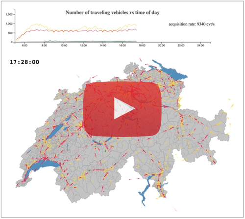
In this post, we propose to walk through an application built to visualize, in fast motion, one day of activity, as shown in this movie. As real time data are not yet available, they were simulated, based on available schedule information. This pretext is too good not to dig into a stack containing Play/Scala/Akka on the backend, Angular2/Pixi.js/D3.js/topojson in the browser, linked together by Server Side Events.
This prototype is intended to explore the possibility of doing massive geographical visualization in the browser, applying techniques described in a previous post.
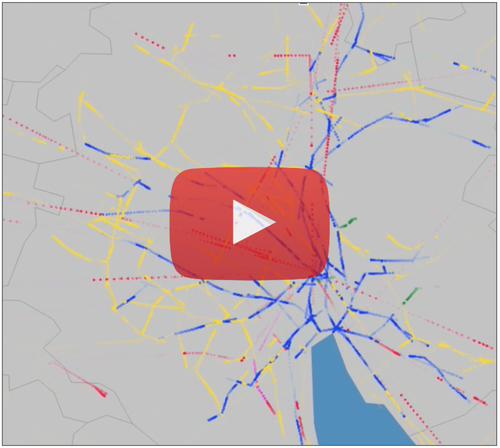
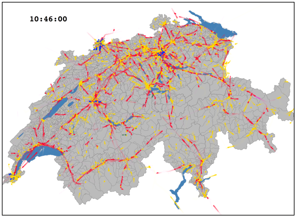
Figure 1: A couple of snapshots linked to Youtube screen recordings.The left figure shows transports across all Switzerland, with a dynamicchart indicating the number of circulating vehicles. The right part is a zoom on Zürich. Red is for trains, yellow for buses, blue for tramways, green for funiculars or gondolas and light gray for boats.The video shows the actual web animation, as the time is “accelerated” on the server side when pushing vehicle positions.
Why this post?
Public transport visualization is well addressed problem. For example, GeOps tracker proposes an impressive tool to dynamically map transit information. Most of the currently versatile solutions are based on schedule information, by opposition to Real Time. Moreover, they usually update vehicle positions by batch to limit traffic: in one HTTP transaction, all the current and forecasted vehicle positions are sent to the browser. Finally, web applications are classically limited to a few tens of vehicles, to cap the load on the infrastructure.
In this article, we remain at the schedule level, but take the opportunity to explore the possibility of asynchronous massive data update: thousands of vehicles see their positions updated independently, opening up to more dynamic interactions.
Beside the transport domain at hand, this prototype is an excuse to explore dynamic visualization.
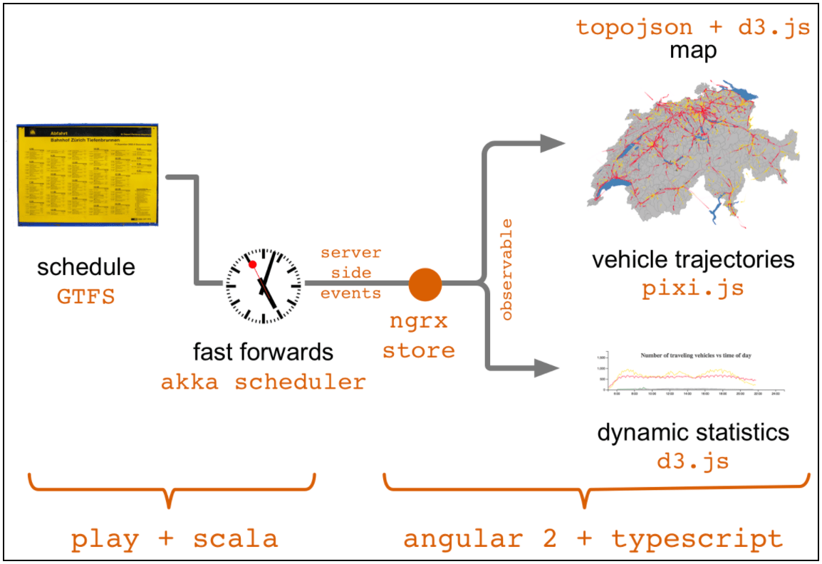
Figure 2: prototype architecture sketch.
Backend: publishing the vehicle positions feed [code]
Scheduled data: the GTFS format
Let’s start with acquiring some data.
The General Transit Format Specification, or GTFS Static, proposes a format to describe a public transport system. This format, created at Google, is widely used, from local companies up to full country layouts. For example, data for the official Swiss schedule are available to download, grouping information for more than 400 companies.
A system comes as a set of .tsv files, typically worth for one year. The full format is described here, but the main components are the files:
agencies.txt: companies running line (~400 elements, e.g. AGS (Andermatt Gotthard Sportbahnen));
stops.txt: localisation names, and geographical coordinates (~30’000, e.g. Jungfraujoch);
trips.txt: route head name (~470’000);
stop_times.txt: a link between a trip, a stop, a time (~8 millions);
calendar_dates.txt: trips and date exceptions;
and more, such as fares, transfer, frequencies information etc.
Being a tabular format, information refer to each other via textual keys.
Our prototype being based on Scala+Akka+Play, we will briefly describe a couple of components.
Playing the schedule
Loading a system
A GTFSSystem, containing all the aforementioned data, is simply loaded into memory at start time from the original text files. For the sake of speed, the versatile tototoshi CSV parser was abandoned, to the benefit of a custom one. In the other hand, to save memory, BitSet were used to handle calendar date exceptions.
Filtering trips
The goal is to play one day of data, so the first obvious goal was to be able to filter trips by date or by agencies (no need to return city transit vehicle on a country wide map). Plotting geographic data also come with bounding coordinates: only trip with at least one stop laying within the viewport bounds are to be reported.Scala collections primitives definitely offer comfortable way to handle such filtering.
Firings playing events
The overall goal is to have simulated position events of vehicle across the day, let’s say every minutes (with some randomization). Based on the GTFS data at hand, we can then interpolate the positions between stops (these interpolations being linear, as the routes actual shapes are not provided). This approximation is a limitation of the simulator not a one of the visualization: with real realtime data, we will receive real positions. Our GTFS system can therefore be transformed into a logbook of vehicle positions, where the time scale can be accelerated (typically by a factor of 500 to play a full day in a couple of minutes),
Actually scheduling these events is the next stone. We used the Akka Scheduler in two layers:
schedule the start event of all the trips simulations across the day;
once a trip is started, it actually schedules all its coming simulated positions.
This two steps approach ensure not to overload the scheduler. Of course, less costly strategies could be put in place to run at a larger scale and lower footprint, but this one proved to be reasonable enough for the sake of this prototype.
On the practical point of view, Akka scheduling consists in delaying the sending of a message to an actor along time. Just to get a taste of it actually working:
simulatedPositionList is the list of simulated positions for a trip;
timeAcc is a time accelerator, transforming a schedule time into an accelerated and relative referential;
actorSink is an actor that will receive all the simulated positions. Where to send them? This question is answered in the next section.
Feeding Server Side Events
One way to stream data from a backend to a web browser are Server Side Events. Well adopted by frameworks such as Angular 2 (see another OCTO post on the matter), they are particularly well suited to handle unidirectional flows, where a browser receives updates from the server
As we’ve seen above, vehicle positions are published across a time window and sent to an actor (actorSink). This actor can then be connected to a Akka stream, used as the the source of the SSE flow. This can be done at the Play controller level.
A naive implementation ties a source to an actor (the one used above as a sink by the scheduler)
val (actorSink, publisher) = Source.actorRef[SimulatedPosition](10000, dropHead) .toMat(Sink.asPublisher(true))(Keep.both).run()
//transform the object stream into JSON stream val jsonSource = Source.fromPublisher(publisher.map(Json.toJson) //the time is accelerated by a factor 500 val timeAcc = TimeAccelerator(500) //launches the event scheduling, //using the ref actor as a sink val actorSimulatedTrips = actorSystem.actorOf( Props(new ActorSimulatedTrips(actorSink, timeAcc, trips)))
//pipe the stream to an EventSource protocol Ok.chunked(jsonSource via EventSource.flow).as(ContentTypes.EVENT_STREAM)
This implementation was named “naive”, as its major flaw is for the akka stream not be closed if ever the HTTP stream is canceled (browser tab is closed, reloaded etc.)
This can be overcome by tying the publisher to a Future: if the stream is closed by the consumer, an ending message can be sent to the publishing actor, so the next scheduled events can be canceled. A code extract:
//ties a Source to a Future def peekMatValue[T, M](origSource: Source[T, M]): (Source[T, M], Future[M]) = { val promise = Promise[M] val source = origSource.mapMaterializedValue { mat => promise.trySuccess(mat) mat } (source, promise.future) }
val (queueSource, futureQueue) = peekMatValue(Source.queue[JsValue](10000, OverflowStrategy.fail))
From the browser side, various high quality JavaScript frameworks are available. ReactJS and Angular 2 certainly are the most prevalent for large data set handling and we opted for the later one, with a Flux architecture and the reactive RxJS libraries.
A classic Angular 2 flux architecture
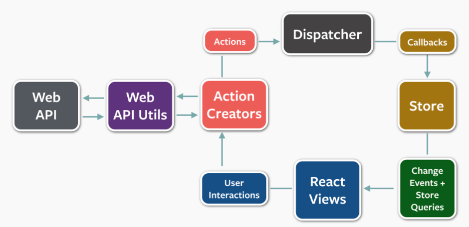
The Flux architecture was originally proposed by Facebook and gained a large popularity with ReactJS, mainly through the Redux implementation. Described in the figure below, the main idea is to handle states in a centralized store. Components register to state change events issued by the store. The store is updated via actions, triggered either by user interactions or external events - in our case, Server Side Events popping in.
Figure 3: Flux architecture schema, by Adobe’s folks.
The store
In our situations, the stored state contains four components:
URL route status (provided by default ) to handle parameters (focus coordinates etc.);
vehicle positions: tied to the SSE stream;
a coordinate system: referring to rendering component size, latitude/longitude boundaries and the associated projection;
metrics: number of events received per second, number of active vehicle per type...
Rendering components and services can then subscribe to store state changes via observable.
At this stage, we are therefore receiving vehicle positions and are able to send them to a rendering component (see details below). However, geographic rendering usually also requires a map.
Geographical concerns
Once more, TIMTOWTDI. Several solutions are available to provide rich map information. The most prevalent certainly are Google Map API, or Open Street Map, without forgetting the more “artistic” versions from Stamen or high quality local systems such as the swiss GeoAdmin API or the french GeoPortail. Even though we have had positive experiences with those systems, we chose for this application the D3 + Topojson approach (check out Mike Bostock’s “command line cartography” post).
Topojson offers an elegant vector based approach, where geographical entities (country, cantons, municipalities, lakes etc. are actually described by independent paths. This presents the advantage of a comfortable rendering with D3.js enter/update/remove pattern, the variety of packaged projections and customization through CSS. Moreover, it also provides a convenient way to link a geographical entity (e.g. canton=Zürich or municipality=St George) to a path, therefore to an optimal scaling on a viewport [code].
Using Topojson & D3.js
We provide a short example of code to demonstrate how a topological feature can be converted to an SVG. The projection referential is used to fit the viewport and can be used to add other features. This later functionality will come handy in the next section, when time comes to append moving vehicles on the map.
svg.attr('width', width) .attr('height', height);
//topoCH is built from here, and get all municipalities const allFeats = topojson.feature(topoCH,topoCH['objects'][municipalities]) .features;
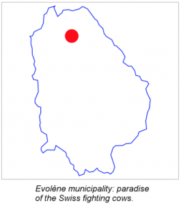
//Just get one municipality const myFeat = allFeats.find((g)=> g.properties.name == 'Evolène');
//Pickup a projection among the dozens available //and adapt it both to the feature and the viewport const projection = d3.geoAlbers() .rotate([0, 0]) .fitSize([width, height], geoJson);
//A function to transform a list of (lat,lng) into an SVG path string const path = d3.geoPath() .projection(projection);
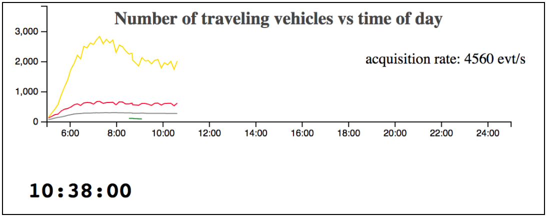
Figure 4: various rendered views: (a) the full country, without city transit (as it is not relevant to be shown at such a scale (Youtube); (b) Zürich city transit (Youtube); (c) a dynamic histogram displaying the count of vehicles across the day and throughput of received events; (d) for the sake of performance measurements, the full country is shown with city transit (although intra city motions are not visible at such a scale).__
Implementation
Vehicles positions are consumed from the SSE stream and stored within a Flux store. Every second or so, the positions can be updated on the screen, with a smooth transition to illustrate the shiftings. Such transition are usually achieved via D3.js selection transitions but performance issues are faced when one handles several thousands of data points.
The solution we used, mixing Pixi.js & d3.js, is discussed at length in a precedent post. It consists in leveraging the power of GPU processing. In the current application, pixi.js will nonetheless use d3.js projection function to convert geographic coordinates into pixels unit.
On the other hand, d3.js is still used to render the map.
Real time statistics, counting the number of vehicles at any given time, are also displayed, as shown in figure 4-c. These numbers are aggregated on the JavaScript side and plotted with d3.js
A few words on performances
Figure 4a shows a video capture for the vehicle transit across the country (without intra city transit), while 4b focuses on the Zürich inner traffic. The full day can be watched on Youtube (a and b). Time is accelerated on the server side, when scheduling the events, while the movie are recorded without any fast forward effect.
No lag can be observed, even when approximately 1500 vehicle positions are updated every second in figure 4-a. In this situation, the server component consumes approximately 35% of one CPU core, while the browser JavaScript consumes 30% and the GPU 40%. The measures were done on a 2015 MacBook pro laptop.
Even if it makes little sense from the visualization point of view (due to the large scale), city transit was added in figure 4d to push the computations limit even further. 4500 vehicles are then observed, with a slight but bearable lag in the point motions. In this situation, CPU numbers are respectively 40/80/70%.
Finally, loading and serving the whole schedule for Switzerland consume 2.5 gigabytes of memory and takes approximately 1 minute to load.
Installation
For the impatient, a packaged application is ready to be ran, with Java 8. Download the latest zip archive from here and unzip it. From within the extracted directory:
#linux/mac bin/gtfs-simulation-play
#windows bin/gtfs-simulation-play.bat
With large data, such as the full Swiss schedule for one year, it can take up to 2.5 minutes to start on a Macbook pro. Then head to your http://localhost:9000 and enjoy!
Head to git to have more details on how to configure the launch, of, for developers, the route to go is to head for git and clone the two application components (front and back), the associated data set and head for the readme files.
Conclusions
We have seen in this post how to render a large amount of moving data on a? map. We believe the presented technique can be used in other situations and pushes further the frontier of rich dynamic data visualization, mixing d3.js and GPU powered framework.
Nonetheless, only a prototype was presented here. Major improvements are yet possible to allow the approach to scale and the footprint on network and CPU to be lowered. The presented scheduling method will hardly scale above a few tens of clients but it could be revisited, or replaced by Kafka once large amount of real time data are to be spread. WebSockets would also allow a more comfortable “dialog” (changing request parameters) and HTTP/2 binary protocol certainly are an interesting promise for lighter and more efficient data exchange.