Using GridGain for Value at Risk calculation
After a first published article introducing the Value at Risk interest and calculation on a Grid, we will now explore the practical implementation by using a grid computing middleware. I have chosen GridGain, an open source grid middleware which implements the map/reduce pattern (see previous article). Firstly, I will give an overview of the Value at Risk implementation independently of the grid computing architecture. Then I will describe the GridGain middleware and the classes that have to be implemented to take advantage of the grid. Finally, I will provide some performance figures from my laptop and analyze how we can improve them.
Some portions of the code were removed for readability reason and replaced by comments (//...). The following class diagram gives an overview of the different classes: 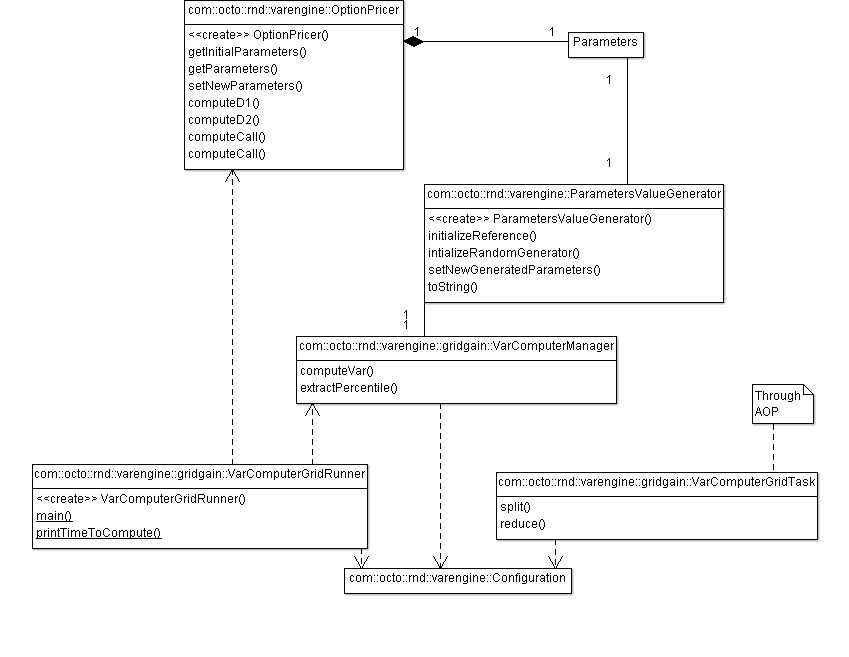
OptionPricer, Parameters and ParametersValueGenerator and VarComputerMaanger are dedicated to the Value at Risk calculation. VarComputerGridRunner and VarComputerGridTask are the classes implemented to take advantage of the grid. Configuration is shared between all layers.
Value at Risk implementation
This simple class computes the option prices according to the given parameters. It is strictly the implementation of the Black and Scholes expression. Mathematical functions like NormalDistribution are provided by Apache commons Math.
public class OptionPricer implements Serializable {
	private static final long serialVersionUID = 5294557359966059686L;
	private static int NUMBER_OF_TRADE_DAY = 252;

	public static class Parameters implements Serializable {
		/**  For Serialization	 */
		private static final long serialVersionUID = -3967053376944712365L;
		/** Time in days before the maturity	 */
		private int t;
		/** Time in year before the maturity  */
		private double tInYear;
		/** Spot (actual price) of the underlying  */
		private double s0;
		/**  Strike (target price) of the underlying  */
		private double k;
		/**  Risk free interest rate  */
		private double r;
		/**  Implicit volatility of the Equity	 */
		private double sigma;

		public Parameters(int t, double s0, double k, double r, double sigma) {//...	}
		public Parameters(final Parameters parameters) { //...	}

		//Getters and Setters...
	}//End Parameters class

	 /** Initialize only one time and reuse the distribution	 */
	private NormalDistribution normalDistribution = new NormalDistributionImpl(0, 1);
	private final Parameters initialParameters;
	private Parameters parameters;

	public OptionPricer(final Parameters intialParameters) {
		this.initialParameters = intialParameters;
		this.parameters = new Parameters(this.initialParameters);
	}
	//Getter and Setter both for initialParameters and parameters...

	/**
	 * d_1 = \frac{1}{\sigma\sqrt{t}} \left[ \ln \left( \frac{S_0}{K} \right) + \left( r + \frac{1}{2}\sigma^2 \right)t \right]
	 *
	 * @param spot actualized by a the yield for this simulation
	 */
	private double computeD1(final double s0) {
		//denominator
		double denom = parameters.sigma * Math.sqrt(parameters.getTInYear());
		//numerator
		//I don't explain - 0.5 * sigma^2 but in the Excel sheet it is like that
		double num = Math.log(s0 / parameters.k) + (parameters.r - 0.5 * parameters.sigma * parameters.sigma) * parameters.getTInYear();
		return num / denom;
	}

	/**
	 * d_2 = d_1 - \sigma \sqrt{t}
	 * @param d1
	 * @return
	 */
	private double computeD2(final double d1) {
		double result = d1 - parameters.sigma * Math.sqrt(parameters.getTInYear());
		return result;
	}

	/**
	 * Compute the price of the call
	 * C(S_0,K,r,t,\sigma) = S_0 \mathcal{N}(d_1) - K e^{-rt}\mathcal{N}(d_2)
	 * \mathcal{N}(x) = \int_{-\infty}^{x} \frac{1}{\sqrt{2\pi}}e^{-\frac{1}{2}u^2} du
	 *
	 * @return
	 * @throws MathException
	 *
	 * @param spot yield Allows to build a actual yield for each simulation
	 */
	public double computeCall() throws MathException {
		final double s0 = parameters.s0;
		final double d1 = computeD1(s0);
		final double d2 = computeD2(d1);
		double result = s0 * normalDistribution.cumulativeProbability(d1) - parameters.k * Math.exp(-1 * parameters.r * parameters.getTInYear()) * normalDistribution.cumulativeProbability(d2);
		return result;
	}
}
Two interesting points can be highlighted. First, for performance reason, I chose to use float point numbers. In order to prevent falling into some pitfalls, some precautions should be taken. No rounding or other non linear function is performed during the calculation. Then all divisions are delayed till the end of the calculation so as to not lower the precision. Then I define both an initialParameters field and a parameter reference for a performance reason which I will explain with the help of the following class.
public class ParametersValueGenerator implements Serializable {
	private static final long serialVersionUID = 2923455335542820656L;
	private final double underlyingYieldHistoricalVolatility;
	private final double interestRateVariationVolatility;
	private final double implicitVolatilityVolatility;

	/** Used to generate the raws */
	private RandomData randomGenerator = new RandomDataImpl();
	/** Reference to OptionPricer initialParameters */
	private OptionPricer.Parameters initialParameters;

	/**
	 * @param underlyingYieldHistoricalVolatility
	 *            Volatity of the yield of the undelying price (it is the
	 *            standard deviation for the normal distribution)
	 * @param interestRateVariationVolatility
	 *            Volatility of the risk free interest rate (it is the
	 *            standard deviation for the normal distribution)
	 * @param implicitVolatilityVolatility
	 *            Volatility of the underlying volatility (we probably take
	 *            the standard deviation of an index like VIX
	 * @see http://en.wikipedia.org/wiki/VIX
	 */
	public ParametersValueGenerator(
			double underlyingYieldHistoricalVolatility,
			double interestRateVariationVolatility,
			double implicitVolatilityVolatility) {
		this.underlyingYieldHistoricalVolatility = underlyingYieldHistoricalVolatility;
		this.interestRateVariationVolatility = interestRateVariationVolatility;
		this.implicitVolatilityVolatility = implicitVolatilityVolatility;
	}

        /**
	    Reseed with a value that is more likely to be unique
		This is mandatory to avoid generating two identical random number series
		To be really sure to not have the same value in two different thread or computer,
		I use a secure random generator instead of the current millisecond

		This method is time consumming, use it a minimum number of times
	 */
	public void intializeRandomGenerator() {
		randomGenerator.reSeed(securedRandomGenerator.nextLong());
	}

	/**
	 * Set the reference
	 * @param initialParameters
	 * @param parameters
	 */
	public void initializeReference(final OptionPricer.Parameters initialParameters) {
		this.initialParameters = initialParameters;
	}

	/**
	 * Put random generated values into parameters instance by modifying it
	 * by reference
	 *
	 * @param parameters
	 */
	public void setNewGeneratedParameters(OptionPricer.Parameters parameters) {
		if(parameters == null) { throw new IllegalArgumentException("parameters should not be null"); }
		if(this.initialParameters == null) { throw new IllegalStateException("this.initialParameters should not be null"); }

		if(this.underlyingYieldHistoricalVolatility != 0) {
			parameters.setS0(this.initialParameters.getS0() * (1+randomGenerator
				.nextGaussian(0, this.underlyingYieldHistoricalVolatility)));
		}
		if(this.interestRateVariationVolatility != 0) {
			parameters.setR(this.initialParameters.getR() + randomGenerator
					.nextGaussian(0, this.interestRateVariationVolatility));
		}
		if(this.implicitVolatilityVolatility != 0) {
			parameters.setSigma(randomGenerator
					.nextGaussian(this.initialParameters.getSigma(),
							this.implicitVolatilityVolatility));
		}
	}
	//toString() method...
}
This class generates random values for the Monte-Carlo method. This simple implementation generates data according to a normal distribution. One interesting thing to notice, from a financial point of view, is the choice of a normal distribution for modeling different values:
- the yield of the strike (leading to
value=initial*(1+nextGaussian())) - the delta of the interest rate variation (
value=initial+nextGaussian()) - the implicit volatility value (
value=nextGaussian())
The setNewGeneratedParameters() method modifies a reference to the parameters reference of the OptionPricer by using a reference to the initialParameters. The initializeReference() method allows to make that reference point to the initialParameters of the OptionPricer. It would have been much easier to return a new Parameters instance for each simulation, but some measures with JVisualVM shows that the Parameters constructor was one of the most consuming method. Indeed, allocating memory on the heap requires looking for the next slot with sufficient memory. This is a costly operation. Passing each generated value to the OptionPricer would probably have been more efficient. But this handling of references seems to be a good compromise between performance and maintainability.
Another interesting point to mention is the intializeRandomGenerator () method. If you do not have it, you will have a strange behavior which could lead to hours of headache. I will describe you the problem and the solution afterwards but before doing so I need to give you some implementation details.
The GridGain tool and the Map/Reduce implementation
This tool brings some functionality allowing executing the code on a grid without coding low level logic. Among the "out of the box" provided functionalities, we can mention:
- Automatic discovery of available nodes
- Deployment of code and data on each node
- Load balancing
- Failover if a node fails or is no more reachable
Concretely, the default implementation of GridGain is very easy to start in a development environment. The only prerequisite is that GridGain is deployed and executed on each node. The written application starts an embedded node. After the auto-discovery, the grid is built as shown in the console (in that case 4 processes on a quad core processor):
>>> -------------------
>>> Discovery Snapshot.
>>> -------------------
>>> Number of nodes: 4
>>> Topology hash: 0xAEFB9485
>>> Local: CD766E36-2A09-45B5-895F-860F5DFBA386, 10.1.106.135, Windows 7 x86 6.1
, mbo, Java(TM) SE Runtime Environment 1.6.0_20-b02
>>> Remote: B5278A02-CD63-4E7E-89FF-BCA791E9045E, 10.1.106.135, Windows 7 x86 6.
1, mbo, Java(TM) SE Runtime Environment 1.6.0_20-b02
>>> Remote: A4201237-6838-44A3-8B32-3E8B5B1F2FFF, 10.1.106.135, Windows 7 x86 6.
1, mbo, Java(TM) SE Runtime Environment 1.6.0_20-b02
>>> Remote: C9BCB5C8-3C87-4106-9E89-8ABF11FEC959, 10.1.106.135, Windows 7 x86 6.
1, mbo, Java(TM) SE Runtime Environment 1.6.0_20-b02
>>> Total number of CPUs: 4
The code is deployed automatically on each node and run.
The map/reduce pattern
GridGain implements the Map/Reduce pattern. This pattern is required to be able to distribute the calculation. In brief, this pattern comes from functional programming. The calculation is broken down into the repetition of the same small calculation on a big number of data (map function). Each small calculation can be distributed. Then the results are merged (reduce function). An in depth description with a sample has been provided in my previous article.
The map/reduce pattern implementation
In this particular case, the code is organized that way. - The VarComputerManager class implements the VAR calculation logic in the computeVar()method. It is not tied to the grid and implements the business logic. To be exact, this method does not return one value but all the values lower than the VAR. See my previous article for more information of the business meaning of the VAR and the calculation algorithm.
public class VarComputerManager {
	/**
	 * Compute the VAR of the option defined in the option pricer
	 * @param optionPricer Instance should be instanciated with the correct parameters
	 * @param valueGenerator Instance should be instanciated with the volatilities, and the reference to the default parameters should have been set
	 * @param drawsNb Number of draws produced on that node
	 * @param totalDrawsNb Total number of draws made on the whole grid
	 * @param varPrecision Between 0 and 1. 0.99 gives the VAR (the percentile) to 1%
	 * @return The n lowest prices generated on that node where n = (1-varPrecision)*totalDrawsNb
	 * @throws MathException
	 */
	public SortedSet<double> computeVar(final OptionPricer optionPricer,
			final ParametersValueGenerator valueGenerator, final int drawsNb, final int totalDrawsNb,
			final double varPrecision, final Configuration configuration) throws MathException {
		final double nbValInPercentile = (totalDrawsNb * (1 - varPrecision));
		final SortedSet</double><double> smallerPrices = new TreeSet</double><double>();

		valueGenerator.intializeRandomGenerator();

		for (int i = 0; i < drawsNb; i++) {
			valueGenerator.setNewGeneratedParameters(optionPricer.getParameters());
			final double price = optionPricer.computeCall();

			// For each draw, put the price in the sorted set
			smallerPrices.add(price);
			if(configuration.isCombineAllowed()) {
				// If the set exceeds nbValInPercentile, remove the highest value
				if (smallerPrices.size() > nbValInPercentile) {
					smallerPrices.remove(smallerPrices.last());
				}
			}
		}

		return smallerPrices;
	}

	/**
	 *
	 * @param smallerPrices Modified by reference
	 * @param drawsNb
	 * @param varPrecision
	 */
	public void extractPercentile(SortedSet</double><double> smallerPrices, final int drawsNb, final double varPrecision) {
		final double nbValInPercentile = (drawsNb * (1 - varPrecision));
		// If the set exceeds nbValInPercentile, remove the highest value
		while (smallerPrices.size() > nbValInPercentile) {
			smallerPrices.remove(smallerPrices.last());
		}
	}
}
</double>
A defined number of draws of random data is executed by the valueGenerator.setNewGeneratedParameters(optionPricer.getParameters()); and the call price is computed for each draw. The lowest values are identified. This example code remains simple by using a SortedSet. One drawback is that if the same VAR is generated by two combination of parameters, the second value will be discarded (add() is an optional operation). In practice, I got this behavior in 0.02% of the draws leading to a potential lower VAR value than expected. For the purpose of that example, I chose to keep that imprecision.
- Then the VarComputerGridTask class implements the technical logic to deploy the code on the grid. The split() function is a synonym for map() of the map/reduce pattern. It defines how to break down computeVar() into smaller functions.
public class VarComputerGridTask extends GridTaskSplitAdapter<gridifyargument , SortedSet<Double>> {
	private static final long serialVersionUID = 2999339579067614574L;
	private static String SESSION_CONF_KEY = "SESSION_CONF_KEY";
	private static Logger log = LoggerFactory.getLogger(VarComputerGridTask.class);
	@GridTaskSessionResource
    private GridTaskSession session = null;

	@Override
	protected Collection< ? extends GridJob> split(int gridSize, final GridifyArgument arg)
			throws GridException {
		// Split number of iterations.
        Integer iterations = ((Integer)arg.getMethodParameters()[2]);

        // Note that for the purpose of this example we perform a simple homogeneous
        // (non weighted) split on each CPU/Computer assuming that all computing resources
        // in this split will be identical.
        int slotsNb = 0;
        //Retrieve the session parameter
        Object[] params = arg.getMethodParameters();
        Configuration conf = (Configuration)params[5];
        //Put it into session to retrieve it in reduce task
        session.setAttribute(SESSION_CONF_KEY, conf);
        if(conf.isThereSeveralSlotsByProcess()) {
        	Grid grid = GridFactory.getGrid();
            for(GridNode node : grid.getAllNodes()) {
            	log.debug("Node {} detected with {} cores", node.getPhysicalAddress(), node.getMetrics().getAvailableProcessors());
            	//1 process per node is presumed. If several processes are running on the machine, the number of cores will be over estimated
            	slotsNb += node.getMetrics().getAvailableProcessors();
            }
            log.debug("{} slots available", slotsNb);
        }
        else {
        	slotsNb = gridSize;
        	log.debug("1 slot by process so {} slots", gridSize);
        }

        // Number of iterations should be done by each slot.
        int iterPerNode = Math.round(iterations / (float)slotsNb);

        // Number of iterations for the last/the only slot.
        int lastNodeIter = iterations - (slotsNb - 1) * iterPerNode;

        List<gridjobadapter <Integer>> jobs = new ArrayList</gridjobadapter><gridjobadapter <Integer>>(gridSize);

        for (int i = 0; i < slotsNb; i++) {
            // Add new job reference to the split.
            jobs.add(new GridJobAdapter<Integer>(i == slotsNb - 1 ? lastNodeIter : iterPerNode) {
				private static final long serialVersionUID = 1L;

				/*
                 * Executes grid-enabled method with passed in argument.
                 */
                public TreeSet<double> execute() throws GridException {
                    Object[] params = arg.getMethodParameters();
                    TreeSet</double><double> result = null;

                    VarComputerManager varComputerManager = new VarComputerManager();
                    try {
                    	result = (TreeSet</double><double>)varComputerManager.computeVar((OptionPricer)params[0],
								(ParametersValueGenerator)params[1],
								getArgument(), //Give the split size on that node
								(Integer)params[3],//Give the total size on the grid
								(Double)params[4],
								(Configuration)params[5]);
					} catch (MathException e) {
						log.error("Error computing option pricing", e);
						result = new TreeSet</double><double>();
					}

					log.debug("{}", String.format("SlotId %d: Map %d elements on %d and produce %d results", this.hashCode(), getArgument(), (Integer)params[2], result.size()));
					return result;
                }
            });//End GridJobAdapter
        }//End for

		return jobs;
	}
</double></gridjobadapter></gridifyargument>
The split() method receives as arguments the size of the grid and a GridArgument object containing the arguments of the VarComputerManager.computeVar() method seen above. The function determines the number of available slots according to the number of processors. As our tasks are computer-intensive, the most efficient repartition is one slot per core. Lets say 1,000 draws can be broken down into 10 tasks applying computeVar() of 100 draws each. For GridGain, a task is represented by a GridJobAdapter instance. In order to be able to measure the influence of different strategies (e.g. one thread but multiple processes or one process and multiple threads per machine), some points have been specified in a configuration object. The GridTaskSession makes it available to each map() and reduce() method. One other tip is to notice that computeVar() has two close but different arguments. The third one -drawsNb- should be equal to 100 on each node but the fourth one -totalDrawsNb- should be equal to 1,000. totalDrawsNb with varPrecision to define the number of values to return: nbValInPercentile = (totalDrawsNb * (1 - varPrecision));. As described in my previous article, it allows each node to return only the 10 lowest prices resulting from their 100 draws. This performance optimization reduces the values sent through the network guarantying as well that these 10x100 values contain the 10 lowest values of the total 1,000 draws.
- The reduce() function merges all the results.
@SuppressWarnings("unchecked")
@Override
public SortedSet<double> reduce(List<gridjobresult> results) throws GridException {
		int nbValInPercentile = 0;
		final SortedSet<double> smallerPrices = new TreeSet</double><double>();

		// Reduce results by summing them.
		for (GridJobResult res : results) {
			SortedSet</double><double> taskResult = (SortedSet</double><double>)res.getData();
			log.debug("Add {} results", taskResult.size());
			smallerPrices.addAll(taskResult);
			Configuration conf = (Configuration)session.getAttribute(SESSION_CONF_KEY);
			if(conf.isCombineAllowed()) {
			//Hypothesis is made that the map task already send only the required values for percentile
				if(nbValInPercentile == 0) {
					nbValInPercentile = taskResult.size();
				}
				else if(nbValInPercentile != taskResult.size()) {
					throw new IllegalStateException("All set should have the same number of elements. Expected " + nbValInPercentile + ", got " + taskResult.size());
				}

				while (smallerPrices.size() > nbValInPercentile) {
					smallerPrices.remove(smallerPrices.last());
				}
			}//End if
		}
		log.debug("Reduce {} jobs and produce {} results", results.size(), smallerPrices.size());
		return smallerPrices;
}
</double></gridjobresult></double>
In our case, the reduce task looks for the 10 smallest values in the 100x10 smallest values sent by each node.
Now lets go back to the parametersValueGenerator.intializeRandomGenerator() method. This paragraph is a bit technical an can be safely ignored by readers who want quickly know how to start the grid
Random number generation issue
When you increase the number of draws, the precision should increase. During my tests, with only one thread, the value was converging normally to 0.19. But with several nodes, the convergence was slower or I got some surprising values even with a high number of draws. Finally, after padding logs everywhere with different parameters I got log containing such lines:
14:21:53.635 [gridgain-#17%null%] DEBUG c.o.r.v.gridgain.VarComputerManager - SO list 125.53733975440497;122.81494382362781;91.27631322995818;108.45186092917872;126.38622145310778; 14:21:53.635 [gridgain-#4%null%] DEBUG c.o.r.v.gridgain.VarComputerManager - SO list 130.49461547615613;113.37411633772678;84.84851329812945;97.68916453583668;126.54608432355151; 14:21:53.635 [gridgain-#6%null%] DEBUG c.o.r.v.gridgain.VarComputerManager - SO list 130.49461547615613;113.37411633772678;84.84851329812945;97.68916453583668;126.54608432355151; 14:21:53.636 [gridgain-#7%null%] DEBUG c.o.r.v.gridgain.VarComputerManager - SO list 130.49461547615613;113.37411633772678;84.84851329812945;97.68916453583668;126.54608432355151;
SO list contains my underlying strike generated values. You can notice that some series are totally identical. The union of these different sets is certainly not a normal distribution as initially expected. Due to the algorithm used and consequently to this, several nodes were sending identical results. And as you may have noticed, these results are aggregated by the SortedSet.addAll() method. Look if required at the JavaDoc of the method and you will discover that elements are optional if they are not already present. So, to summarize, N nodes with total identical values are equivalent to one unique node. No doubt possible, the results are totally wrong. But why?
To understand it, we need to know how commons math RandomDataImpl works. The javadoc gives us a clue by saying "so that reseeding with a specific value always results in the same subsequent random sequence". The default implementation I used is based on the Random class of the JDK. The algorithm used to generate random values is called Linear congruential generator. To summarize, it is a mathematical series %20%%20n) that, given an initial value called seed, builds a list of numbers that have the properties of a normal distribution. To give a practical image, it is close to - even though very different in mathematical properties - to the Mandelbrot set where a mathematical formula can lead to something random, chaotic.  (Source http://en.wikipedia.org/wiki/Mandelbrot_set#Image_gallery_of_a_zoom_sequence) However, if you give twice the same seed to a generator, it will generate the same list of values. Writing the following
 initializeRandomGenerator function
public void intializeRandomGenerator() {
	randomGenerator.reSeed(2923455335542820656L);
}
leads to that kind of log: all lists of generated values are identical.
14:51:28.781 [gridgain-#10%null%] DEBUG c.o.r.v.gridgain.VarComputerManager - SO list 105.61456308819832;105.61456308819832;105.61456308819832;105.61456308819832;105.61456308819832;
14:51:28.781 [gridgain-#14%null%] DEBUG c.o.r.v.gridgain.VarComputerManager - SO list 105.61456308819832;105.61456308819832;105.61456308819832;105.61456308819832;105.61456308819832;
14:51:28.781 [gridgain-#12%null%] DEBUG c.o.r.v.gridgain.VarComputerManager - SO list 105.61456308819832;105.61456308819832;105.61456308819832;105.61456308819832;105.61456308819832;
14:51:28.781 [gridgain-#13%null%] DEBUG c.o.r.v.gridgain.VarComputerManager - SO list 105.61456308819832;105.61456308819832;105.61456308819832;105.61456308819832;105.61456308819832;
By default, the seed used by Random class is the current timestamp. I have tried to use a mix of the thread identifier and System.nanoTime() but I still got some strange behavior. The easiest fix was to define this initializedRandomGenerator.
private SecureRandom securedRandomGenerator = new SecureRandom();
//...
public void intializeRandomGenerator() {
		randomGenerator.reSeed(securedRandomGenerator.nextLong());
	}
SecureRandom is designed for cryptographic scenario and uses a different implementation that guarantees better randomness. But in counterparty, it is much slower than the standard Random class. So this method initializeRandomGenerator() is called once at the beginning of the computeVar() method to provide the seed, then the standard class is used. This solution fixes the problem. However, it is only a quick answer for the purpose of this article. I have not checked that the union of the generated random lists corresponds to a normal distribution. Further analysis, comparison with other random generators (see this Wikipedia article) should be useful for a real world use case.
Grid instanciation
Finally, after resolving that problem, we can look at the VarComputerGridRunner that instantiates the master node of the grid.
public final class VarComputerGridRunner {
	//...
	/**
	 * Method create VarEngine and calculate VAR for a single Call
	 *
	 * @param args
	 *            Command line arguments, none required but if provided first
	 *            one should point to the Spring XML configuration file. See
	 *            <tt>"examples/config/"</tt> for configuration file examples.
	 * @throws Exception
	 *             If example execution failed.
	 */
	public static void main(String[] args) throws Exception {
		conf = Configuration.parseConfiguration(args);
		// Start GridGain instance with default configuration.
		if (conf.getGridGAinSpringConfigPath() != null) {
			GridFactory.start(conf.getGridGAinSpringConfigPath());
		} else {
			GridFactory.start();
		}

		resultsLog.info("VAR\tDrawsNb\tComputeTime (ms.)\tParameters");

		try {
			//Compute multiple times, until 2 min. or 10^6 (32 bits heap size limit)
			double maxTime = System.currentTimeMillis() + 2*60*1000;
			for (int i = 1000; i < 100000001 && System.currentTimeMillis() < maxTime ; i *= 10) {
				VarComputerManager varComputer = new VarComputerManager();
				OptionPricer.Parameters params = new OptionPricer.Parameters(
						252, 120.0, 120.0, 0.05, 0.2);
				OptionPricer op = new OptionPricer(params);
				ParametersValueGenerator valueGenerator = new ParametersValueGenerator(
						0.15, 0, 0);
				printTimeToCompute(varComputer, valueGenerator, op, i);
				valueGenerator = new ParametersValueGenerator(0.15, 0.20, 0);
				printTimeToCompute(varComputer, valueGenerator, op, i);
				valueGenerator = new ParametersValueGenerator(0.15, 0.20, 0.05);
				printTimeToCompute(varComputer, valueGenerator, op, i);
			}

		}
		// We specifically don't do any error handling here to
		// simplify the example. Real application may want to
		// add error handling and application specific recovery.
		finally {
			// Stop GridGain instance.
			GridFactory.stop(true);
			log.info("Test finished");
		}
	}

	private static void printTimeToCompute(
			final VarComputerManager varComputer,
			final ParametersValueGenerator parametersValueGenerator,
			final OptionPricer optionPricer, final int drawsNb)
			throws MathException {
		double startTime = System.nanoTime();
		parametersValueGenerator.initializeReference(optionPricer
				.getInitialParameters());

		final double varPrecision = 0.99;
		SortedSet<Double> smallerPrices = varComputer.computeVar(optionPricer,
				parametersValueGenerator, drawsNb, drawsNb, varPrecision, conf);
		//If combine is not allowed in Map/Reduce, all results are brought back
		//Extraction of percentile should be done here
		if(!conf.isCombineAllowed()) {
			varComputer.extractPercentile(smallerPrices, drawsNb, varPrecision);
		}
		double var = smallerPrices.last();
		double endTime = System.nanoTime();
		resultsLog.info("{}", String.format("%f\t%d\t%f\t%s", var,
				drawsNb, (endTime - startTime) / 1000000, parametersValueGenerator.toString()));
		log.info("{}", String.format("%f (computed with %d draws in %f ms.) with generators %s", var,
				drawsNb, (endTime - startTime) / 1000000, parametersValueGenerator.toString()));
	}
}
When GridFactory.start() is called, the GridGain middleware starts the master node which looks for other nodes and builds the grid. GridGain default configuration uses multicast for nodes discovery but other implementations are available. Then, when varComputer.computeVar() is called, the GridGain middleware calls transparently the VarComputerGridTask class through Aspect Oriented Programming. The split method breaks down the calculation, produces several calls to VarComputer.computeVar() with different parameters. The middleware sends code and data to the nodes. Each node executes VarComputer.computeVar(). Then the results are sent back to the master node. The master node executes the reduce() function before returning to main(). In my example, the main() function has to
- First extract the percentile if not done by map/reduce;
- Then identify the real VAR value: the highest value of the computed set.
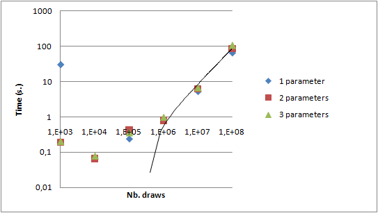
Some performance figures
With that implementation it is now possible to experiment some performance measures. I used my laptop, a DELL Latitude E6510 with a core i7 quad core and 4 GB of RAM. 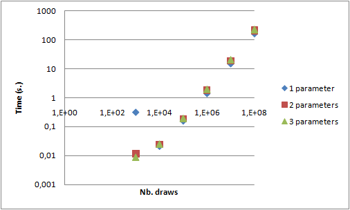
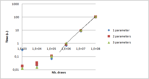
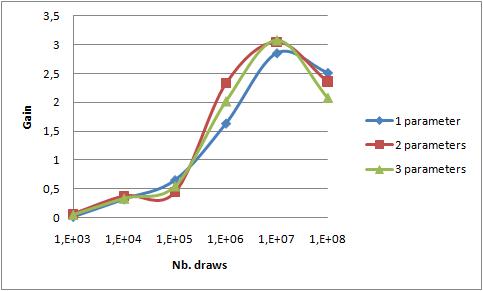
Gain between 1 thread and 4 threads is not visible on such graphs. The following graph draws that gain in two cases:
- 4 jobs launched on 4 threads in a single process (
Configuration.isThereSeveralSlotsByProcess=true,VarComputerManageris launched alone) - 4 jobs launched on 4 processes (
Configuration.isThereSeveralSlotsByProcess=false,VarComputerManageris launched with 3 other GridGain.bat processes)
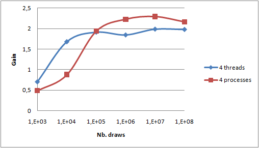
First, as expected, the gain is higher for a higher number of draws. So distribution should only be used for more than 10,000 draws in our example. Secondly, we can notice that the gain is less than 4: between 2 and 2.5. Several main reasons can be invoked:
- My Core i7 has two physical cores and Hyper-Threading technology allowing 4 threads. So even though the OS sees 4 processors, only 2 are physically available. Performance gain made available by Hyper-Threading is according to that Wikipedia article 30% and not 100% as we presumed by expecting a total gain of 4. This Intel article goes much more into details but quotes gains up to 70%. So 4 threads should lead to a maximum expected gain between 2x1.3=2.6 and 2x1.7=3.4. The Intel article specifies that extremely computing efficient applications are more likely to have smaller gains with Hyper -Threading. It is globally the case of that sample application which is computing intensive and with very little memory sharing due to the "combine" optimization - i.e. sending only 1% of the total number of draws to the
reduce()function.- - Only the
maptask can be distributed. In that particular algorithm,reduceis time consuming - Distribution comes at a cost
Third, the gain is slightly higher for threads with few draws and higher for processes with many draws. As the differences are not very marked, it could be due to measure imprecision. If I had to formulate an hypothesis, I would guess that JVM and OS best pin processes to core leading to better cache utilization.
Then I used a second laptop from a colleague: a Dell Latitude 34800 with a Core 2 Duo and 2GB RAM. Both were connected on our internal (shared) wire network through a switch. Because of the different number of cores, the default homogeneous repartition of jobs by GridGain leads to 3 jobs on each PC. This behavior can be changed programmatically as shown in that example. To bypass that problem, I launched 6 jobs in 6 processes (Configuration.isThereSeveralSlotsByProcess=false).
VarComputerManageris launched with 3 other GridGain.bat processes on my laptop- 2 GridGain.bat processes are launched on the other laptop
- Distribution on different machines comes at a greater cost than local distribution;
reduce()function - not distributed - is higher because more results are built simultaneously by 6 map tasks;- Gain has been computed with the 1 thread reference on the Core i7. Comparisons by Intel made on two different versions of Core i7 and Core 2 Duo shows that ratio is about 1.5. So, a rough estimation of the maximum expected gain could be 2x1.3+2x0.66=3.9 which is rather close to 3.
In conclusion, distribution comes at a cost. So distribution should be limited to computing with a high number of draws. Optimizations of that code leads globally to correct performance gain.
All previous measures have been made with "combine" option (i.e. sending less data to reduce()) activated. In order to estimate the benefit of that optimization, take a look at the 2 following graphs. They show the relative gain after activating the "combine" optimization both on 4 threads on local PC and on 6 processes on two PCs.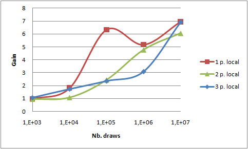
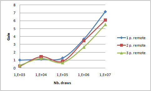
reduce() function - brings a gain of 7. This value is the same in both cases, so we can assume that network bandwidth saving is not the key point here. Measures on my laptop with no "combine" option shows a maximal network throughput of 11.6 MB/s on my 100MB/s network interface. The network interface output queue length remains to 0 confirming that point. So I conclude that reducing the workload of the reduce() function leads to that gain.
Conclusion
Grid middlewares like GridGain provide valuable functionalities in order to implement VAR computation using Monte-Carlo method through the Map/Reduce pattern. However, despite their efforts, code should be written with a distributed deployment in mind. The random generators should be managed to remain accurate. Transferring configuration or other information requires adapting both the technical code and the interface of the business code. Moreover, optimizations are required to provide good performances. Lowering the work of the Reduce() function leads in my case in a x7 gain. Finally, distribution comes at a cost. This cost is higher between machines than between local processes. The distribution over-head is made profitable for a high number of draws, so the granularity of the distribution should be tuned. This simple example provides relatively good gain due to the simplification made and consequent optimizations. In a real world scenario, intermediate results are frequently stored in order to be further analyzed. Implementing such use case will be the next challenge and the purpose of my next article.