Time series features extraction using Fourier and Wavelet transforms on ECG data
ABSTRACT
This article focuses on the features extraction from time series and signals using Fourier and Wavelet transforms. This task will be carried out on an electrocardiogram (ECG) dataset in order to classify three groups of people: those with cardiac arrhythmia (ARR), congestive heart failure (CHF) and normal sinus rhythm (NSR). Our approach consists of using scaleogram (i.e. 2D representation of 1D extracted features) as an input to train a Neural Network (NN). We conducted the different tasks using python as a programming language. The results presented at the end are satisfactory and demonstrate the pertinence of the approach.
INTRODUCTION
Many data science problems e.g. weather prediction, stock market analysis, predictive maintenance, etc. comes with data that vary over time. We refer to those data interchangeably as time series (TS) or signals. Then we can apply the same extraction techniques for TS than for signals. Whether it is for the classification or regression tasks, the feature extraction is an important step that will influence the accuracy of the intended predictions.
In this article, we first present the pros and cons of using Fourier transform and wavelets on an ECG dataset. Then, we explain how a 2D view of the extracted 1D features can be used as an input image to train a Neural Network.
An ECG is a graphical representation of the electrical activity of the heart, in other words it is an electric signal that varies over time. Usually an ECG was limited to a medical environment but recently some smartwatches capable of performing an electrocardiogram appeared on the market. This kind of signal seems a good example to start with a basic review of Fourier and Wavelet transforms.
In order to gain some insight on the data we first begin by exploring the ECG data set which contains data collected from people classified into three groups, those with cardiac arrhythmia (ARR), congestive heart failure (CHF) and normal sinus rhythm (NSR) as shown in Figure 1.
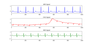
Figure 1: Representation of the three classes of ECG in our data, in line blue arrhythmia (ARR), in red congestive heart failure (CHF) and normal sinus rhythm (NSR) in green.
Methodology
In this part, we will present our methodology based on Fourier Transform (FT) and Wavelets_(1)_ to extract features in order to classify the signals in three different classes: cardiac arrhythmia (ARR), congestive heart failure (CHF) and normal sinus rhythm (NSR).
Beforehand, we should distinguish between continuous and discrete time signal in order to apply a discrete or continuous Fourier Equation. If the signal is a continuously occurring phenomenon, then we can represent it as a function of a time variable 𝑡 thus, 𝑥(𝑡) is the value of signal 𝑥 at time 𝑡, its domain is a subset of the real numbers. We speak then of a continuous signal.
However, for a discrete-time signal, values are only defined at specific time-steps, it will be defined for example at every second, t = 1 s, t = 2 s, t = 3 s. In our ECG example we deal with a continuous signal, so in the following we show how to apply Fourier Transform and Wavelets on this continuous signal.
(1) It is worth to mention that these two techniques are the visible part of the iceberg because signal processing is a widespread field, Book.
Fourier Transform
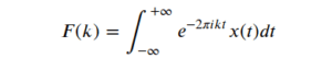
Fourier analysis was developed to study periodicity in a signal and the main idea of this technique is to decompose the signal in its periodic components. Periodicity is a basic concept when it comes to signals, it means if the signal contains a pattern, which repeats itself after a specific period of time, we call it a periodic signal. The time it takes for a periodic signal to repeat itself is called the period 𝑃, and the inverse of the period is named as frequency, 𝑓, for a signal with a period of 1 sec, its frequency is 1 Hertz (Hz). Therefore for a periodic signal the definition for the continuous Fourier transform F(k) of the time-domain description of a signal noted as 𝑥(𝑡) is defined by:
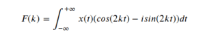
Thanks to the Euler formula the equation (1) can be written in a different format using sine and cosine functions as :
After applying a Fourier transform on a signal we will obtain information about the component frequencies of the signal, F(k) in our notation. At this step we usually speak about space of frequency or frequency-domain description.
The aim of applying Fourier transform is to decompose the original signal into a sum of its simpler signals, no matter how complex the original one looks. We refer to simpler signals, as the trigonometric functions sine and cosine. In general when we move from a signal in the time-domain to frequency-domain we speak of direct Fourier transform (FT) in the opposite case to change from frequency to time the equation is called the Inverse Fourier Transform.
To illustrate the later equation with an example we will use a synthetic data set where we include a number of individual frequencies [2, 5, 3]. In Python, the FT of a signal can be calculated with the SciPy library in order to get the frequency values of the components of a signal.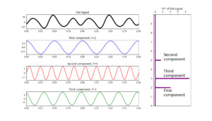
Figure 2: Synthetic data, in first horizontal box we plot the full signal in black, next boxes in lines red, blue and green are the individual components, corresponding to frequencies of 2, 5 and 3 respectively. In the vertical box we show the result of Fourier transform.
In Figure 2 the black line corresponds to the full signal built as a linear combination of trigonometric functions plotted in lines blue, red and green, with frequencies 2, 5, and 3, respectively. From the original full signal these frequencies are unknown at this stage, just after Fourier transformation we get the frequency spectrum that compose the full signal, as plotted in purple in the vertical box.
Towards a classification model:
Going back to the example of the synthetic signal where it allows a clear decomposition in Fourier transform, we propose to collect all maxima positions peaks from the frequency domain, for example using the scipy library peaks, and use them as features.
Doing that, the labeled signal ‘synthetic’ will have a row of associated maximum positions, here the peaks are easily identified as peak_1: (x_1=2, y_1=4 ), peak_2: (x_2=5 , y_2=1.5 ), peak_3: (x_3=3 , y_3=9 ).
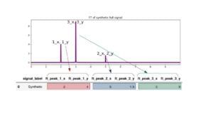
Figure 3: Schema representing the technique to extract features from a Fourier transform.
Following the notation on the above table means that feature ft_peak**_1_x** is the x coordinate of the first frequency for the signal, and feature ft_peak**_1_y** is the y coordinate; feature ft_peak_2_x is the x coordinate of the second frequency detected and so on. Then our features in the example for the labeled 'synthetic' signal are : ft_peak_1_x , ft_peak_1_y , ft_peak_2_x, ft_peak_2_y, ft_peak_3_x, ft_peak_3_y .
In the case where our data set of signals allows a clear frequency identification we can feed a dataframe to train a classification algorithm.
We can improve the problem description by adding more features exploring other signal processing techniques (concerning signal processing techniques you can delight with a large list of them in scipy.), like power spectral density (PSD) represented by the magnitude squared of the Fourier Transform. Even more, we can add statistical features like average, median, and variance of values. All these will be translated as more columns in the data frame.
Having transformed the dataset into an exploitable data frame the next step is to choose a classifier algorithm to train, nevertheless we will continue with the study of another technique that best suits our data, follow us!
Let us try the FT with a real signal extracted from the ECG dataset. In Figure 4 we plot as full signal an arrythmia example followed by its Fourier transform.
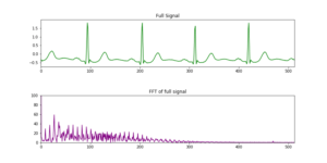
Figure 4: ARR ECG as full signal in green line, below FT result in purple color.
In contrast to the very well defined set of frequencies obtained with synthetic data, in Fig. 4 the FT is less clear, we managed to identify some peaks but in some intervals they are not sharp. Why Fourier is not able to break down the signal clearly? To answer this we should pay attention to time. In the synthetic case we have a signal composed by three frequencies, and these frequencies are fixed on time, they do not vary. Fourier transform works when no variation in time happens, when we are in the frequency-domain we lose this dependency. In some way we can think of the Fourier transform as a trade-off between time information and frequency information. By taking a FT of a time signal, all time information is lost in return for frequency information. Our ECG signal is full of frequencies that vary on time, that is the reason why we can not resolve it clearly in frequency domain.
Wavelets
We saw in the last section that we need a method to handle signals whose constituent frequencies vary over time (e.g. the ECG data). We need a tool that has high resolution in the frequency domain and also in the time domain, that allows us to know at which frequencies the signal oscillates, and at which time these oscillations occur.
The Wavelet transform fulfils these two conditions. In order to solve the problem of loss of knowledge from the temporal domain, the Wavelet transform modifies the shape of the simple sine and cosine functions of the Fourier transform. In a Wavelet the mother function is finite in time in contrast to Fourier where sine and cosine run from (-∞,+∞). Unlike a Fourier decomposition which always uses complex exponential (sine and cosine) basis functions (see Eq. 1 and 2), a wavelet decomposition uses a time-localized oscillatory function as the analyzing or mother wavelet, as shown in Figure 5.
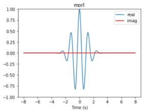
Figure 5: Real Morlet mother function.
For a continuous signal, 𝑥(𝑡) from one dimension, its transformed Wavelet into a 2D space is defined as:
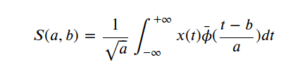
Being a a scale factor and b a translation factor applied in the continuous mother wavelet .
We will call the wavelet by its mother wavelet name, for example shan for a Shannon kind function, and by two other parameters a and b , as in the case of shan1.5-1.0 in the first box of Figure 6, where a = 1.5 and b = 1.0. b, is the central frequency parameter used to build the wavelet and it is related to the period by period = s/b , where s corresponds to the scale, it can be any array of values in increasing order. a, is associated to the bandwidth_parameter which selects how much the wavelet is sensitive to the frequencies around b. For complex mother functions, we show an example in the second box in Figure 6, where the mother wavelet cgau3 represents cgau for the complex Gaussian mother function and the number 3 is associated to the order of the derivative of the wavelet function.
In summary, if we have a dynamical frequency spectrum, in other words if our signal has frequencies that change in time, then we need a tool with resolution not only in the frequency domain but also in the time domain, a Wavelet. In short, we should catch that wavelet transform is an efficient tool for analysis of short-time changes in signal morphology.
Before to apply a wavelet transform on our ECG data set, let us a minute to show you what kind of functions we can find as a mother wavelet. A big difference with the Fourier transform, where sine and cosine are used as basis functions is that for wavelets we have a family of them:
'Haar', 'Daubechies', 'Symlets', 'Coiflets', 'Biorthogonal', 'Reverse biorthogonal', 'Discrete Meyer (FIR Approximation)', 'Gaussian', 'Mexican hat wavelet', 'Morlet wavelet', 'Complex Gaussian wavelets', 'Shannon wavelets', 'Frequency B-Spline wavelets', 'Complex Morlet wavelets'.
The choice of a particular mother function will depend a lot on the signal to be treated, we can even create our own wavelet function.
As can be expected the Wavelet Transform comes in two different and distinct flavors; the Continuous and the Discrete Wavelet Transform similar to Fourier.
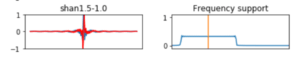
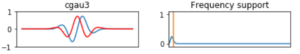
Figure 6: Some of the members of the family wavelet functions used to compute the transform. First column are wavelet functions, second column corresponds to description of a and b parameters.
Now we are ready to see in action a wavelet transform applied on one of the signal of our ECG dataset. For better visualizing the transformation we will use an 𝑠𝑐𝑎𝑙e𝑜𝑔𝑟𝑎𝑚, a tool that build and displays the 2D spectrum for Continuous Wavelet Transform (CWT). An scalogram takes the absolute value of the CWT coefficients of a signal and plot it.
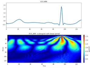
Figure 7 : Top box corresponds to an interval of ECG signal class: ARR, the box below is the results after applying a Wavelet transform with a Morlet wavelet.
Before diving into a machine learning subject it is worth understanding the scaleogram output. In vertical axe we plot the period (defined above), in the horizontal axe we show the scale, there is a relationship between scale and period mediated by the central frequency, a parameter of the chosen wavelet, frequency = b/s.
We can interpret each horizontal characteristic in the scaleogram as a frequency of the total signal. The fact of not seeing a continuous line in our figure corresponds to that said frequencies are not continuous in time.
A very relevant point to our exercise is the fact that the scaleogram can be understood as a picture, an image as any other and then apply a model like NN to train a classifier as we will show you in the next section.
Application
Training the ECG classifier with scaleograms
Interpreting ECGs is often difficult, then automatic interpretation of ECGs is useful for many aspects of clinical and emergency medicine, for example in remote monitoring, as a surgical decision support or in emergencies. In this section we perform a classification, as a rapid method of disease identification. The fact of transforming ECG signals into scaleograms allows us to use a visual computing model to classify the different types of diseases in our data set. As any image we can decompose the scaleogram in RGB spectra. An important fact to note is that each row is an ECG recording sampled at 128 hertz, this means that the scaleogram of a single signal-component produces an image of 127 by 127 pixels.
Our data contains ECGs from three groups of people, ARR, CHF, NSR, the first two correspond to diseases and the third group are healthy people. To classify these groups, we propose to use basic neural network using TensorFlow 2.0, so we keep in mind that our images have a format 127 pixels to our input shape and decompose in 3 filters due to RGB, then our model has the following characteristics:
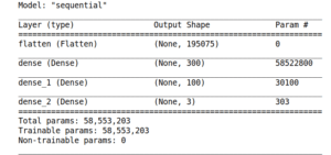
Figure 8: Schematic representation of our Convolutional Neural Network.
After running 10 epochs using a stochastic gradient descent as optimizer, and computing the loss with a sparse categorical cross-entropy, the accuracy metric shows a very good performance, as shown in Figure 9.
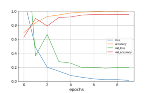
Figure 9: Learning curve for 10 epochs, in blue and green lines we plot loss and validation loss, in orange and red we plot accuracy and validation accuracy.
Last step to consolidate our model is to explore one metric more appropriate to a multi-class problem, the confusion matrix, represented in Figure 10.
A Confusion matrix gives us a good idea of the performance of a classification model. Each line corresponds to a real/true class, each column corresponds to an estimated/predicted class. We compare true values against predicted values, then for good models we should expect a high number of elements in the diagonal, where all elements predicted correspond to the real ones. In our case we normalized the confusion matrix, so the maximum value expected in the diagonal is 1. From Figure 10 we can see that our model predict very well all the three classes because all values in the diagonal are very close to 1.
After transforming our ECG data into scaleograms we reach a very good classification result for the three groups of persons. Now, if you have a smartwatch that performs ECG, at least you can know in which of these three groups you are, cross fingers in NSR. But remember, a doctor's advice is always recommended!
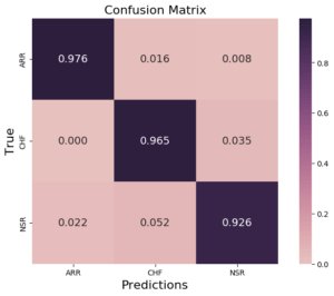
Figure 10: Normalized confusion matrix plot for classification results obtained with the CNN previously defined in Figure 8.
Conclusion
In this article we have seen two different ways to extract features from signals based on time dependence of frequency distribution, Fourier and Wavelet transforms. These functions transform a signal from the time-domain to frequency-domain and give us its frequency spectrum.
We have learnt that Fourier transform is the most convenient tool when signal frequencies do not change in time. However, if the frequencies that make up the signal vary over time, the most performant technique is a wavelet transform. The last case allows us to explore the frequency domain of the signal as an image by formatting the output as an scaleogram and then take advantage of image classification techniques. Based on ECG data, we made a classification over three groups of people with different pathologies: cardiac arrhythmia, congestive heart failure and healthy people. With a very simple neural network we were able to get a precise model which quickly allows us to detect a healthy person from others with heart disease.
Next steps :
We believe that this work is the starting point to a large study of ECG signals, next steps can be the cleaning of real signals and the inclusion of other pathologies in order to enlarge the classification scope of diseases. We also propose the use of low pass and/or high pass filters to clean the signal.
In parallel the study of sound waves as ultrasound can be explored with theses techniques and of course anything that you challenge.
Code: https://github.com/mnf2014/article_fft_wavelet_ecg/blob/develop/wavelet_article_octo.ipynb
Links of interest:
https://github.com/alsauve/scaleogram/blob/master/doc/scale-to-frequency.ipynb
http://ataspinar.com/2018/12/21/a-guide-for-using-the-wavelet-transform-in-machine-learning/
http://nicolasfauchereau.github.io/climatecode/posts/wavelet-analysis-in-python/
https://towardsdatascience.com/what-is-wavelet-and-how-we-use-it-for-data-science-d19427699cef