The evolution of bottlenecks in the Big Data ecosystem

le 12/10/2015 par Benjamin Joyen-Conseil, Oliver Baillot

I propose in this paper a chronological review of the events and ideas that have contributed to the emergence of Big Data technologies of today and tomorrow. What we can see regarding bottlenecks is that they move according to the technical progress we make. Today is the JVM garbage collector, tomorrow will be a different problem.

Here is my side of the story:

The early days of the web

The Web era has dramatically changed things in term of data. We have progressed from a rather rigid model of RDBMS that was designed for the IT management (inventory management, accounting) to IT content, extremely diversified and in large quantities:

At the beginning, Google’s index referenced 26 million web pages (in 1998).

Assuming that a web page weighs 100 Ko at the time, we can estimate at 2.5 TB the data volume to index! Two years later, the volume index already exceeded 100 To ...

A quote by Nissan Hajaj, an engineer at Google Search, symbolizes this awareness:

“We’ve known it for a long time : the web is big.”

First observation: Scalability

Google needs to combine two elements so its idea can work

A high computing power
A large power storage

At the time, two ways existed for intensive computations:

The super computer (eg. IBM with Big Blue)
Computer cluster

The first uses the principle of scale-up, in other words: just add RAM and CPU on the motherboard to increase the power.

The second applies the principle of scale-out, add a machine in the cluster to increase its power. It is found under the term horizontal scalability.

Second observation: the variety of information to be processed

The content of sites that Google must index is highly variable.

Indeed, HTML produces pages all very different (in size, content, etc ...). It is not conceivable to store it in an RDBMS designed to handle specific types with a fixed size (INTEGER, VARCHAR (255), timestamp, etc ...).

To anticipate the evolution of the Web, it is necessary to not define any structure, any type, at the moment of the data storage in order to change the structure seamlessly.

We therefore need a system that Google knows how to interpret when the data type is read, instead of defining it when it is written. A sort of brute force to perform Web indexing batches.

Parallelization techniques

One is said shared memory paradigm. This is the case in a single machine that owns multiple CPUs (or cores). CPUs share the same RAM memory in which they access.

The other paradigm is said distributed memory. We have several machines, each one with its own memory. The idea is to transfer information at each step. A loop runs on each machine, and at each iteration, there is a synchronization mechanism to communicate information between machines (Message Passing).

In the clustering case, the strategies used with Message Passing for the distribution and the data retrieval (scatter, gather, broadcast, reduction) use a master node with dataset and workers (running nodes). The data will be downloaded and processed over the cluster, then the result will be retrieved on the master.

MPI strategies

If the first solution to process our dataset is to communicate over the network, the network will form a bottleneck for a data-intensive workload.

Doing the math quickly: (26 million pages * 100 KB in size) / 100 Kbits bandwidth per second / 60s / 60min / 24h = 2.5 days of data transfer.

At the time, these kind of problems rarely occured. MPI (Message Passing Interface) was the library used for intensive computing, it was not designed for large data processing. But according to Google, it is a new use case that is not treated by any existing solution.

Google’s treatments (compute the PageRank, building a reverse index) are long-term processing. Within a distributed environment, the probability of a failed treatment increases with the number of machines running parallel processing. This means that Google should think about a way to tolerate the error (known as fault tolerance).

From these successive observations, Google has been inspired by functional programming to create a new approach within a distributed environment: MapReduce

Use case 1: Batch processing to index the Web

The basic principle is to remove this bottleneck known as the network: Moving binaries, rather than the data.

Instead of distributing the data at the reading stage, we will distribute the data at the writing stage over multiple machines. At the reading stage, there will be only the compiled code that will transit over the network instead of 10TB of HTML pages.

Moreover, the MapReduce paradigm aims greatly to simplify the writing of parallel programs. Progress existed so MPI could co-locate data but it never really materialized because it was not very intuitive and added more complexity.

The fault tolerance is easier to implement: when the data is written, the data is then replicated to different locations. In case of a machine failure containing the information, we will be able to perform our treatment on the replicated data.

Hadoop

Hadoop came in 2006. To build itself, Hadoop requires a distributed file system Nutch File System (currently HDFS), and an implementation of Google MapReduce’s paper. The framework is written in Java, the simple reason is: “Java is portable, easy to debug and widely acclaimed by the community”, said Doug Cutting, its main creator.

With MapReduce, we are using another data-model to represent our recordings: key/value. The perks of this model is its simplicity to be distributed. Each machine gets a key sequence to manage. It is easy to iterate in parallel over each key and perform a treatment on the value. The number of sequences defines the degree of parallelism (number of machines which process a parallel sequence).

// map phase. Ce code est exécuté sur chaque worker
while(recordIterator.hasNext) {
    record = recordIterator.next;
    map(record.key, record.value);
}

The user (developer MapReduce) only needs to specify the purpose of the map() méthod.

The new pairs of key/value generated by the mappers are then distributed to the reducers through the network. This sending stage is called the “Shuffle & Sort”. enter image description here

We can notice that MapReduce is not really a complete solution regarding network issues. Indeed, the shuffle & sort stage mainly uses the network as an exchange medium output data of the map stage to the reducers. The good practice to adopt in the mappers is to filter records, plan (reduce the number of columns), pre-aggregate and compress to significantly reduce the data travelling over the network in the next phase. Unfortunately, these practices are applicable only in individual cases, it is difficult to find a comprehensive solution to this problem.

Use case 2: iterative processing for analytics

Around 2008, we begin to see a new use case: the need for a higher level of language to express a distributed processing. A language designed for the data, the SQL.

Facebook develops Hive, a SQL engine generating MapReduce in 2009. Google introduced Dremel, a distributed datastore interpreting SQL and "optimizing" the full scan (fun), which will give birth to the project Apache Drill (worn by MapR). Impala, Presto, Apache Phoenix, Druid, Pinot, are all so many technologies that will address this need of large volume analysis.

In short, the Analytics is the new use case.

Meanwhile, we begin to see tests in the field of artificial intelligence. The Machine Learning is entering in the Hadoop ecosystem with Apache Mahout and opens new perspectives that stimulate the specialized press.

These two new possibilities on Hadoop (analytics and machine learning) have a common characteristic: they consist of iterations.

Thus, an SQL query is made of several joints that will be split into multiple MapReduce jobs, storing the intermediate result on HDFS. A clustering algorithm such as K-means proceeds by successive iterations until the centroids reach a steady state. They are given the name of iterative algorithms.

At the end of each MapReduce iteration, we store the intermediate result on HDFS for the next iteration. Not only we stored on any hard drive, but the data will be replicated (3 times by default). Then, in the next iteration the intermediate data need to be reload in memory (during the map) to send them directly to the reducers (with shuffle!). It turns out that HDFS is a rather slow abstraction (30MB / s write, 60MB / s average read SATA) that just increase the overall processing time.

As you would have guessed, I/O disks are the new bottleneck.

This bottleneck already existed in reality, but it was masked by the I/O network, and it was not too painful for batch processing.

To minimize the impact of an iteration, we will do what we usually do when we have a need to read / write the data quickly: cache in RAM.

Random Access Memories :

enter image description here

Fortunately, the price of memory has dropped a lot and it is common for some time to find servers with 128 or 256 Go of RAM.

So we can imagine that a dataset of 1TB (replicated) could be hold in memory on a small cluster of about 12 servers…

That is how, the research paper). The Framework is introduced by UC Berkley to solve precisely this type of iterative workload. They think about an abstract data model going through the iterations: the RDD (Resilient Distributed Dataset paper)

An RDD is a collection of records, distributed across a cluster, recovered from a context initialized at the beginning of the job.

//records représente un RDD JavaRDD<String> records = spark.textFile("hdfs://...");

Transformations or actions are successively applied. These two concepts, specific to the Spark’s vocabulary can be generalized by what is called a transaction. It exists map side operators and reduce side operators (shuffle operator). The difference between one and the other is that the reduce side is an operator type that triggers the shuffle (redistribution phase by the network of key / value pairs) before the execution. Spark is not the only abstraction based on MapReduce, most of the frameworks, dataflow type (to express a sequence of transformations) use these same concepts: Apache Flink, Apache Crunch, Cascading, Apache Pig, etc …

records.filter(...) // est une opération map-side
records.groupByKey() // est une opération reduce-side

With Spark, one action generates a run with a shuffle phase.

There are different types of RDD, some offering caching functions particularly to clarify that a dataset will be used on several iterations (thus hiding the intermediate results). The dataset will be stored either in a local cache in RAM or on disk or shared between RAM and disk.

records.cache();

But this is not the only factor of intermediary time acceleration. Spark recycles "executors" - the JVMs used to execute treatments – cleverly. We realized that some of the Hadoop latency was coming from the JVM’s startup. Recycling enabled to reduce the time processing of 20 seconds per iteration (in the Hadoop case, a container takes 30 seconds to initialize). The trick was already in Hadoop (the property mapred.job.reus.jvm.num.tasks in the Hadoop v1 configuration) but was not by default enabled.

With improvements in terms of latency by recycling JVMs and through the use of caches, we begin to see more and more interactive systems. Spark offers an interactive console (bin/spark-shell) to type and run code (Scala and Python languages).

Use case 3: Interactive queries

It is a kind of iterative algorithm. SQL, as we have seen, has become an important point on Hadoop. The shortcut quickly made about Big Data technologies supporting SQL, will be to compare the latency with older systems which themselves used SQL (but processing small volumes): under an average of one minute to display the result of a query.

Business teams, analysts, BI engineers have access to all that power so they can “interact” with the data and extract value.

Hive – with initiatives such as Stinger and Stinger.next – are moving in this direction. It offers new runtimes environment, more suited to the “interactive” (Tez, Spark) to decrease processes on adhoc queries.

The challenge of these new analysis engine (Spark, Flink, Tez, Ignite) is able to store very large amounts of data in memory. We therefore increases the size of the JAVA Heap containers (Xmx the options ans Xms JVM). It will take more RAM. From 2 to 4 GB on average for MapReduce, it will grow to 8 or 16GB for Spark, Tez and Flink. For I/O disk, they will be reduced by increasing the Heap simply because we had the ability to store more objects in memory.

Interactive processing therefore lead to more substantial memory sizes to manage for the JVM, although many small objects are allocated (dataset records), frequently (with every new adhoc query).

We find ourselves in a new bottleneck: the garbage collector

GC limits

The JVM‘s garbage collector is a very powerful mechanism, greatly facilitating the management JVM’s memory (Heap). It automates the deallocation of unused objects.

To manage its objects, it is a graph wherein a node represents an object, and an arc connected to another node corresponds to a reference (an object that references another). If an object has no arc connected to itself, it means it is no longer referenced by any other object, so it can be deallocated when the next collection occurs (it is "marked"). Logically, time travel of the objects collection is proportional to the number of existing objects in the Heap, and therefore the size of the Heap (the bigger it is, the more you can put in).

The garbage collector puts the whole system on hold in some cases (concurrence issue).

Here are some examples causing pause:

Resizing the Heap (it oscillates between Xms and Xmx)
Garbage collection (GC compaction)
Promotion of objects in the generation Tenured
Tagging live objects
etc…

If you are interested to dig deeper the GC process, Martin Thompson gave a very good explanation.

In the diagram below, we see that breaks completely stop the system to complete their treatment, whether performed in parallel or not. It is also called STW pauses, standing for Stop The World. enter image description here

Spark collections are often composed of millions or billions of records, represented by instances. All these fast allocations and deallocations are fragmenting a lot the memory. enter image description here

The garbage collector is triggered at a frequency which varies depending on the use of the Heap. If it no longer offers enough memory to requests for allocation, the garbage collector will conduct a collection to free up space. If it is too fragmented, the JVM will perform a compaction following a collection.

These passages are sometimes too long for the interactive (imagine 30 seconds of GC pause). That is why the main current work on performance Spark is about the garbage collector. Daoyuan Wang's company Databricks (main contributor Spark) gives an overview of possible tweaks in a post titled “Tuning Java Garbage Collection for Spark Applications”.

Philippe Prados raises the question of the future of the GC in a previous article Blog OCTO: The next death of the garbage collector? "Today, the configuration has evolved enough to put the garbage collector on. Incremental developments, which are real, respond less and less to requests. GC are evolving, but not fast enough in relation to their environment.”

This is why engineers will start looking for solutions elsewhere…

How to fool the GC?

In distributed data systems processing (using Java technology), we observe two variants to try to reduce the impact of garbage collection in the JVM.

Hide objects during garbage collector
Use the native memory rather than the Heap

Both variants use the same JDK class: the ByteBuffer A ByteBuffer is a type of object that encapsulates an array of bytes with access methods. The binary information is serialized in advance before storing it into the ByteBuffer. It is a kind of low-level container, in which we will store our collections of objects. According to the documentation, there are two types of ByteBuffer: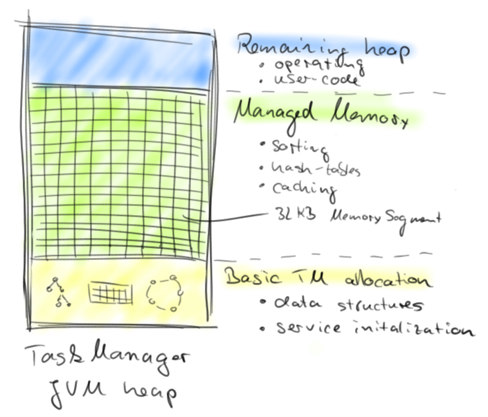

Non-Direct ByteBuffer is a buffer allocated in the Heap up to a maximum size of 2GB. The Non-Direct ByteBuffer is used to conceal the object references in the GC. All our objects are serialized (e.g instances of records in Spark) and then inserted side by side in some Non-Direct ByteBuffer having the role of page, memory segment. Thus, there are only ByteBuffer which are found in the reference graph that travels the GC (it means fewer items). It allocates ByteBuffer when the application is starting, it is arranged that they occupy a fixed portion of the Heap (often 70%). They are long-lived objects, so the JVM does not have many allocations during processing (memory remains stable). And as the memory capacity are reserved to start, there is no resizing the Heap.The diagram refers to an area of the Heap called "Managed Memory" divided into 32K MemorySegment. These Memory Segment are ByteBuffer.
**Direct ByteBuffer a**s its name suggests, accesses the native memory directly. The native memory? You get it, this ByteBuffer is not allocated in Heap but in the memory of the operating system (OS), the mechanism underlying is no more than calls to the Unsafe API. Therefore, the Direct ByteBuffer is not managed by the garbage collector and objects serialized either inside (this process is also called "off-heap"). The Javadoc recommends the use of it for large buffers and long term. The ByteBuffer should be managed by the program that calls it, which brings us to the fact that if an error occurs then the program will crash, throwing an exception BufferUnderflowException. An error can quickly arrive because the ByteBuffer has no method size() so you just have to know the size of its memory objects (varying depending on the hardware) to allocate new objects beside, without rewriting above, or without exceeding the buffer. His second asset is not to copy the buffer content to an intermediate buffer when accessed.

The GC is not put aside. It always manages de-serialized objects and temporary structures that the user allocates in its program (the developer who uses the Spark API).

Flink Management Memory

Flink first implemented the first solution, e.g the use of Non-Direct ByteBuffer allocated in the Heap. The ByteBuffer are called MemorySegment, they are fixed to 32 KB in size and are managed by the MemoryManager. The purpose of this one is to distribute good operators segments (filter, join, sort, groupBy, etc ...).

Flink plans to migrate to the second method: the use of off-heap memory to further accelerate access (no copy in a temporary Buffer) and almost completely bypass the garbage collector (there is always the de-serialized object stored in the Heap).

With these new tricks (the ByteBuffer), serialization is the mechanism that becomes the most important thing. That is why it becomes important to develop serializers for each object type. Flink includes serializers "homemade", but the task is rather heavy (what about Java generics that converts any Object type?) And users classes are serialized from a serialization based on reflection (Kryo), though less powerful than the version "homemade".

SPARK-7075: Tungsten Project

Spark plans to catch up on Flink by launching the Tungsten Project, and for the latest version (1.4) incorporates an interesting mechanism to generate "custom-serializer" code. Code generation facilitates the life of the developer while being much more specific than using libraries such as Kryo.

They are only at the beginning but the project plans to incorporate a MemoryManager with memory pages in the manner of Flink in the version 1.5, and the appearance of efficient structures using the processor caches (L1, L2, L3).

The shared cache, the next bottleneck?

ByteBuffers are very useful but they have a big flaw is that they are costly in terms of serialization / de-serialization (even with custom-serializer). Frameworks such as Flink and Spark spend their time performing these tasks to access their records. To remove the load of systematic de-serialization of objects in the operators, we are starting to see data structures called "cache aware". In other words, a structure able to efficiently use the shared cache of the processors.

The model is: Storing a contiguous collection of key + pointer in a ByteBuffer. When an operator (join, groupBy, sort, etc ...) performs the comparison between the records, it does it on the keys. It is therefore more interesting to separate the value from their value (often larger). Keys have a fixed size which makes the looking of collection effective without de-serialization (you remember the RDBMS at first, it's the same thing). We will do a binary comparison between the keys (or the first bytes of string keys type) and access the value only when it is needed. This access is made via the pointer near the key. Once the bytes retrieved from the ByteBuffer, we de-serializes into an object.

The following chart summarizes this explanation: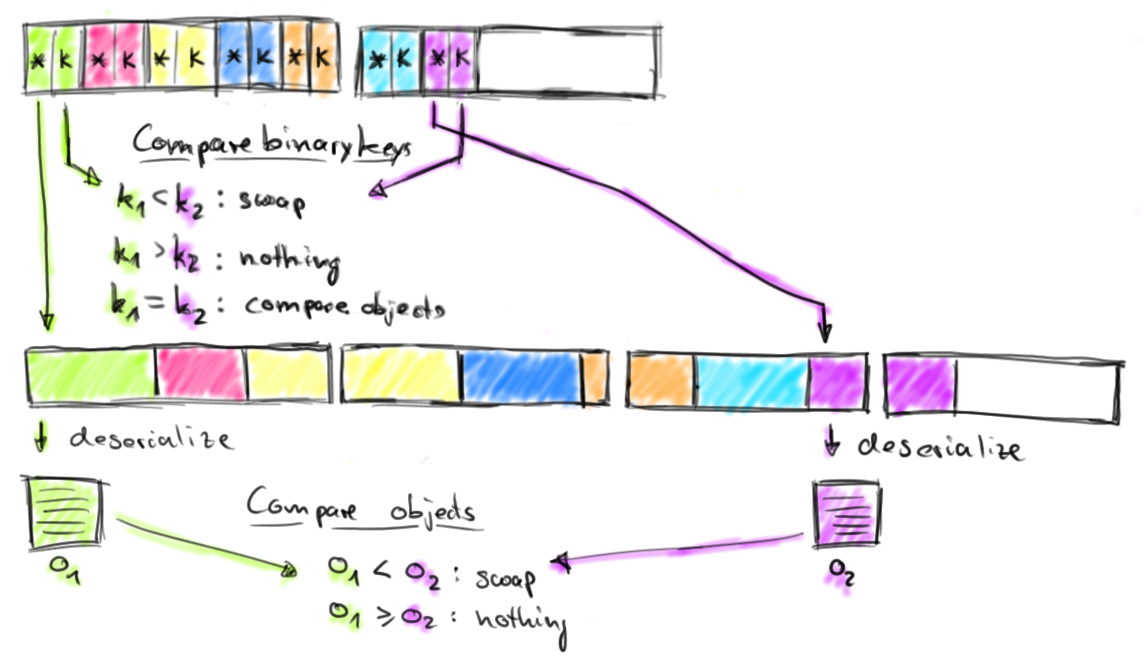

Why these structures are "cache aware"? In fact, these structures are accessed very frequently, and they use little memory (because they have only got keys and pointers), so the OS will place them in the shared cache of the processors (L1, L2 , L3).

This is the end

By analyzing all this, I made the following reflection:

Seeing all these efforts to bypass the garbage collector, we are entitled to wonder why we use a platform whose main asset is to offer a managed memory, if it is to avoid using it?

In practice, the user using frameworks such as Flink and Spark has the best of both worlds. These frameworks limit the impact of GC for their internal mechanics, optimizing the management of large data sets, making them extremely powerful. But they allow developers to use a high-level language, abstracting them of memory management, which is a strong argument towards their utilisation.

Solve bottleneck problems, it is like starting over and over again (infinite loop). Even before Spark has incorporated these evolutions, we can already bet a coin on the fact that the shared cache of the processor will be the next bottleneck of big data systems. Quoting Carlos Bueno: Cache is the new RAM

The future will tell us how to get around it...