Let’s code: Drift and Detect!
The goal of this article is to induce together various types of concept drifts on the UCI Wine dataset as well as understand and test different drift detectors. The code and GitHub repository is provided. A vos claviers!
Did you say drift?
This is Part 2 of the Drift Article series. If you want to learn more about Concept Drifts and Detectors, please read the previous article here.
Let’s say that you are part of the Data Science team of a wine company. You worked on a model to predict wine quality. With promising results (80% accuracy), you decide to put your model into production. However, a few months later, you face a severe drop in the model’s accuracy (50% accuracy).
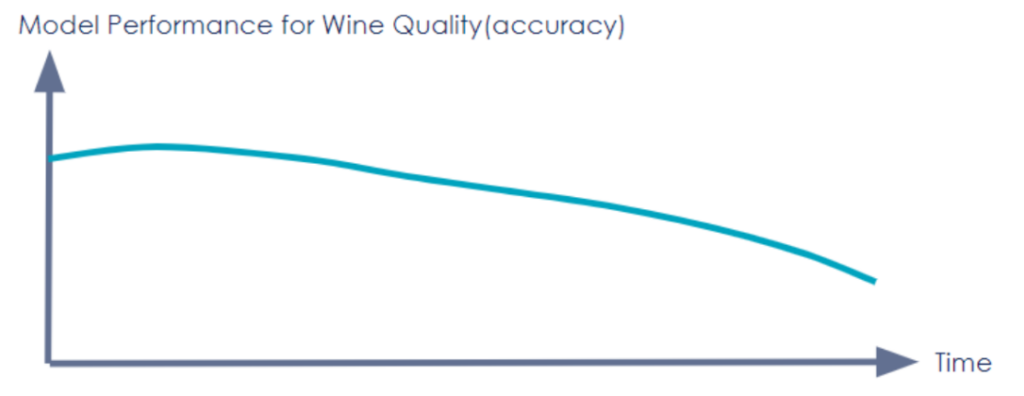
A drop in a model’s performance is only the tip of the iceberg: it can have various explanations. One of them is concept drift.
A concept drift happens when the data you used to build your Machine Learning model changes with time. In other words: it is not representative of the world as it was when first built.
There are two main types of concept drifts: virtual and real.[10]
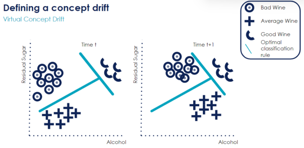
A virtual concept drift happens when the data shifts but the relationship between the target variable and its predictors remains the same. Let’s take an example with our wine quality classification problem: we use two variables (Residual Sugar and Alcohol) to classify a wine as “Bad”, “Average” or “Good”. We can see that between time t and time t+1, some points have drifted to the right (more alcohol). In other words, the alcohol feature has changed. Yet, there has been no change in the optimal classification boundary: this is why it is called virtual concept drift.
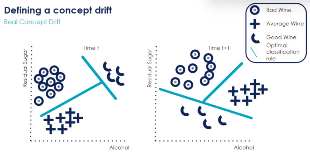
In contrast, real concept drifts disrupt the optimal classification rule: the relationship between the target variable and its predictors has changed. For instance, in the previous plot, data points classified as “Good Wine” had lots of sugar and alcohol. However, at time t+1, data points classified as “Good Wine” only have little sugar and alcohol. This shows a real concept drift because previously, we could see a positive correlation between the target variable “Quality” and its predictors “Residual Sugar” and “Alcohol”. Now, the correlation is negative: the less sugar and alcohol, the better the wine.
We can also classify drifts as abrupt, gradual, or recurrent. If a concept drift happens very quickly in time, it will be called abrupt. In contrast, if it happens slowly, it will be called gradual. Finally, drifts can also repeat themselves: they will be called recurrent. For more information about those drifts, please refer to the previous article of the series here.
A quick word about the Github and Code
The Github repository can be accessed here. You will find several Jupyter Notebooks and scripts.
The content description can be found in the README file.
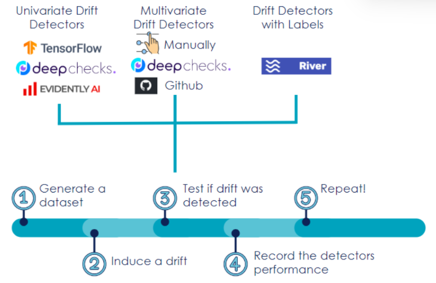
The Drift Detection Framework
Let’s introduce our Drift Detection Framework. It contains several steps, from generating a dataset, to inducing a drift and detecting it in a chosen dataset. Drift simulation is an important step in order to gain confidence in our drift detection methods.
We will go through each step in more detail.
Generate a dataset
Here, we assume that data comes in batches. Data can also come as a stream, but this will not be covered in this article.
In our wine quality use case, we take random samples of the UCI Wine dataset.
Induce a drift
We will now induce drifts on the random sample we have just generated.
Using the UCI Wine dataset, let’s illustrate how to induce two types of drifts: a virtual concept drift and a real concept drift. Three features of the UCI Wine dataset will be used: residual sugar, alcohol, and wine type.
Virtual Concept Drift
The goal is to change a feature’s distribution. There are several ways to do this:
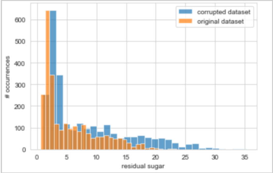
- For numerical variables, you can play with the feature distribution: increase all values of a feature by 10%, or decrease them by a value of 2. In the below example, we decide to multiply the residual sugar values by 50%:
wine_dataset_corrupted_residual_sugar = drift.drift_generator_univariate_multiply(data=wine_dataset_test, column_name=”residual sugar”, value=1.5)
The below plot illustrates the values of the “residual sugar” column for both the original and corrupted dataset. Can you see how values have drifted?
- For categorical variables, you choose to swap values. For instance, when the wine type is characterized as “white”, we change it to “red”.
wine_dataset_corrupted_wine_type = drift.drift_generator_univariate_categorical_change(data=wine_dataset_test, column_name='wine_type',value0="white", value1="red")
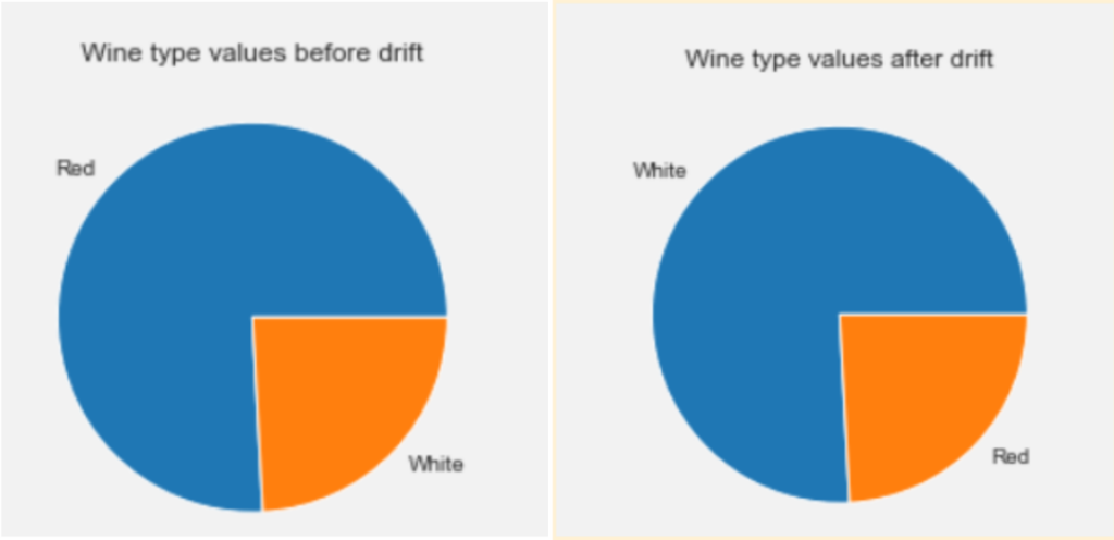
As the previous pie charts shows: the value count for red and white wines are now swapped.
There are also many other ways to induce virtual concept drifts: you can refer to the python file drift.py on the Github repository to try something else.
Real Concept Drift
To induce a real concept drift, we need to find a way to change the relationship between the target and the dependent variables. Some suggestions:
Look at a feature importance graph and induce a virtual concept drift on an important feature. For instance, if we know that the sugar level feature is highly significant, we can change its distribution in order to disrupt the optimal decision boundary
Change the relationship between a covariate and the target variable. For this, we can look at their correlation. Let’s say that the more alcohol in the wine, the higher the quality. Then, we will select the data points where alcohol is high and update their label to “Bad” wine
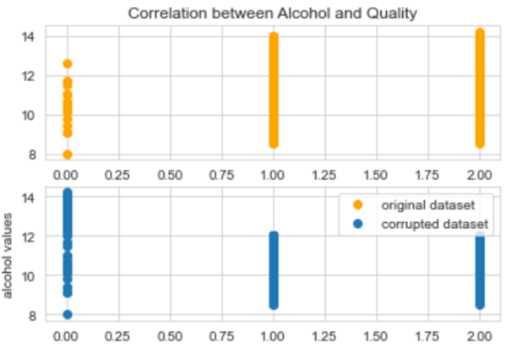
In the below example, we go with Option 2: change the relationship between the alcohol level and quality.
wine_dataset_corrupted_concept_drift = drift.drift_generator_concept_drift(data=wine_dataset_train,label_col="quality",label_value=0,column_name="alcohol",value=12,action="greater")
As we can see from the below plots: the correlation between Alcohol and Quality in the corrupted dataset is different from the correlation in the original dataset. Look at the trend: in one plot, it is a positive correlation and in the other one, it is negative.
For real concept drifts, what’s most important to remember is that the classification boundary has to change.
Other types of drifts
It is also possible to simulate gradual or recurrent drifts. You can find examples of those drifts in the Jupyter Notebook Workshop_MLENG_concept_drifts_.ipynb
Test if the drift was detected
We will now use various detectors to test if our drifts are detected. Let’s first find out more about those detection methods
Overview of the drift detection methods
We can group drift detectors into three main families: univariate drift detectors, multivariate drift detectors, and drift detectors with labels. The below table gives an overview of the three families:
| Family Name | Description | Examples | Tool Used |
| Univariate Drift Detectors | Detects drifts by going through each feature and comparing the new batch distribution with the training distribution | 2-sample Kolmogorov-Smirnov Test [5] <br>Wasserstein Distance [11] | Evidently AI <br>DeepChecks <br>Tensorflow Data Validation |
| Multivariate Drift Detectors | Detects drifts by looking at the covariates (not feature by feature) and comparing them with the training distribution | Margin Density Drift Detector Method (MD3) <br>OLINDDA <br>Hellinger Distance Based Drift Detection Method (HDDDM) | Github and literature articles |
| Drift Detectors with Labels | Detects drifts using labels by looking at the model performance (called error rate) | Early Drift Detection Method (EDDM) <br>Hoeffding Drift Detection Method) (HDDM_W) <br>ADaptive WINdowing (ADWIN) | “River” Python package |
Univariate Drift Detectors
They are widely available on the cloud, private and open-source platforms. We have chosen three open-source platforms: DeepChecks [12], EvidentlyAI [4] and TensorFlow Data Validation [3].
They all use different statistical methods (for example: 2-sample Kolmogorov-Smirnov Test) to detect drifts based on various criteria: whether the feature is numerical or categorical, the sample size, sensitivity of the detector, etc.
If you are interested in finding out more about which statistical method to choose, stay tuned: it will be covered in the next article of the series.
The code implementing those three detectors can be found below:
Multivariate Drift Detectors
They are less used in industry and more of a research topic. We have implemented OLINDDA [9] manually from statistical papers and used Github repository code for the remaining two multivariate methods: MD3 [8] and HDDDM [2].
What is interesting is that those three detectors use very different techniques to detect concept drifts:
OLINDDA [9] uses clustering methods: if a new cluster (a grouping of data points) is formed in a new batch, it is likely that a concept drift has happened. It is implemented in this file: drift_detector_multivariate_ollindda.py
MD3 [8] uses the change in the number of samples within the “zone of uncertainty” of a detector. In other words: for a classification task, if samples are close to the decision boundary, they are “uncertain”. If we see a rise of “uncertain” samples, it may mean concept drift. You can refer to the python file here: drift_detector_multivariate_hdddm.py
HDDDM [2] compares the Hellinger distance (similarity between two probability distributions) between the old and new batches. If it is higher than a threshold, we raise a drift alarm. The link to the code is there: drift_detector_multivariate_md3.py.
Drift Detectors with Labels
Drift Detectors with labels can be implemented using the “River” python package. They are only detecting drifts that have an impact on the model’s performance. Indeed, those methods compare the ‘true labels’ with the model’s prediction. If a difference is spotted such as there are much more errors in the new batch than in the training batch, an alarm is triggered.
We use three different detectors:
Hoeffding Drift Detection Method - HDDM_W [7] it averages the data to give less weight to the oldest data.
Early Drift Detection Method - EDDM [6] uses the distance between two consecutive errors to detect if drift has occurred.
ADaptive WINdowing - ADWIN [1]: uses sliding windows to monitor error rates.
Three drift detectors with labels are implemented in the drift_detector_with_labels.py file.
You can now test to see if any of those detectors can detect the drifts we have induced. Below is some code to illustrate how to use them.
Example Code to detect a virtual concept drift
In the three code snippets, we use the previously induced corrupted dataset (“wine dataset corrupted residual sugar”).
Example Code for Univariate Detectors
DeepChecks_detectors.DeepChecks_detect_drift(wine_dataset_train, wine_dataset_corrupted_residual_sugar,label_col="quality", cat_features=categorical_features_names, model=lgbm_model, test_type="feature_drift")
Example Code for Multivariate Detectors
drift_detector_multivariate_md3.md3_detect_drift(wine_dataset_train,
wine_dataset_corrupted_residual_sugar,label_col="quality")
Example Code for Detectors with Labels
data_merged = pd.concat([wine_dataset_train, wine_dataset_corrupted_residual_sugar], axis=0)
data_merged = data_merged.reset_index(drop=True)
drift_detector_with_labels.drift_detector_with_labels_test(data_merged,label_col="quality", model = lgbm_model,test_name="EDDM")
Record the performance & Repeat with other drifts and other detectors!
Is my 50% increase in residual sugar detected?
We now aggregate the performance of all detectors regarding the virtual concept drift of a 50% increase in residual sugar.
First of all, we determine success as
The drift was detected
There were no false alarms (mistakenly detects a drift in another feature)
For some detectors, there is a distinction between “Warning” and “Alarm”. A warning means that a concept drift can potentially happen very soon whether an alarm detects that a concept drift is happening.
| Drift Detector | Drift Detected | False Alarms |
| DeepChecks Feature Drift | Detected - Warning | None |
| Evidently AI Data Drift | Detected - Alarm | None |
| Tensorflow Data Drift | Detected - Alarm | 9 |
| EDDM | Detected - Warning and Alarm | None |
| HDDM_W | Detected - Warning and Alarm | None |
| ADWIN | Detected - Alarm | None |
| HDDDM | Not Detected | None |
| MD3 | Not Detected | None |
| OLINDDA | Not Detected | None |
Comments:
Many detectors have succeeded in the detection of the drift without false alarms.
The univariate detectors (DeepChecks, Evidently AI, Tensorflow Data Validation) have all raised an alarm for the feature ‘Residual Sugar’. However, one of them: Evidently AI has also raised many false alarms. It means that it wrongly detected drifts in other features.
The detectors with labels (EDDM, HDDM_W, ADWIN) have all successfully detected the drift (both Warnings and Alarms). It means that this 50% increase in Residual Sugar has severely impacted the performance of the model.
Finally, the multivariate drift detectors (HDDDM, DM3, OLINDDA) have not detected the drift. One explanation could be that the drift did not result in a change in the repartition of the data points (no new cluster, no additional “uncertain points).
Is my real concept drift with Alcohol detected?
| Drift Detector | Drift Detected | False Alarms |
| DeepChecks Feature Drift | Not Detected | None |
| Evidently AI Label Drift | Detected - Alarm | None |
| Tensorflow Data Drift | Not Detected | 10 |
| EDDM | Detected - Warning and Alarm | None |
| HDDM_W | Detected - Warning and Alarm | None |
| ADWIN | Detected - Alarm | None |
| HDDDM | Not Detected | None |
| MD3 | Not Detected | None |
| OLINDDA | Not Detected | None |
Comments:
Detecting a real concept drift is more difficult because it can or cannot result in a change in feature distribution. If we have access to the true label values, we can check if the label distribution has changed. This is what we have done with Evidently AI and it has detected the concept drift.
The drift detectors with labels all have detected the real concept drift. It makes sense because the relationship between a feature (alcohol) and the label (quality) has changed. Therefore, the performance of the model has changed.
Finally, the three multivariate drift detectors have not detected the concept drift either. This is because the feature distributions have not changed: the real concept drift cannot be detected with those methods.
Lastly, we will end with the analysis of the performance of gradual virtual concept drift.
Test for a Gradual Virtual Concept Drift : increase sulphates value gradually everyday by 0.1
Example Code for Univariate Detectors
DeepChecks_detectors.DeepChecks_detect_gradual_drift(data_train=wine_dataset_train, data_to_compare=wine_dataset_test,label_col="quality", cat_features=categorical_features_names,model=lgbm_model,
action="increase",value_drift=0.1,column_name="sulphates",test_type="feature_drift",nb_sample=100, nb_days=5)
Example Code for Multivariate Detectors
drift_detector_multivariate_md3.md3_gradual_drift(data_train=wine_dataset_train,
data_to_compare=wine_dataset_corrupted_residual_sugar,column_name="sulphates",label_col="quality",model=lgbm_model,value_drift=0.1,action="increase",nb_sample=100,nb_days=5)
Example Code for Detectors with Labels
drift_detector_with_labels.drift_detector_labels_gradual_drift(data_train=wine_dataset_train,data_to_compare=wine_dataset_test,column_name="sulphates",label_col="quality",model=lgbm_model,value_drift=0.1,action="increase",test_name="EDDM",nb_sample=100,nb_days=5)
| Drift Detector | Drift Detected | False Alarms |
| DeepChecks Feature Drift | Warning Day 0 then Alarm for the remaining days | None |
| Evidently AI Data Drift | Alarm for all days | Many false alarms |
| Tensorflow Data Drift | Alarm for all days | Many false alarms |
| EDDM | Not Detected | None |
| HDDM_W | Not Detected | None |
| ADWIN | Not Detected | None |
| HDDDM | Not Detected | None |
| MD3 | Detected at Day 3,4,5 | None |
| OLINDDA | Not Detected | None |
Comments:
The results are drastically different from the previous drifts!
First of all, except for Deepcheek, the univariate drift detectors did not perform very well: many false alarms were raised.
Secondly, no drift detector with labels was able to detect the gradual concept drift. A possible explanation is that the slight increase in sulphates did not have an impact on the model’s performance. Therefore, the drift could not be detected.
Lastly, the drift was detected by a multivariate drift detector: MD3 for the three last days. It means that from day 3 onwards, the drift was important enough to impact the number of uncertain samples in the margin.
A quick word about parameters
All the previous detectors have been implemented with their default parameters. For instance, the warning values for Evidently AI or DeepChecks are set at 0.1. Therefore, it is important to remember that those results can always be improved by tuning the parameters. One way to do it could be by looking at historical data or comparing different parameter values and finding the best one. By best, we mean the parameter value allowing the most accurate drift detection with the least number of false alarms.
However, we should be careful: drifts can severely affect a dataset so a parameter optimal at time t may not be optimal anymore at time t+1.
Conclusion
Congratulations, you have successfully induced drifts on the UCI Wine Dataset and leveraged different detection methods to detect those drifts!
The key takeaway from this article:
There are several ways to induce virtual and real concept drifts.
There are also several methods able to detect those drifts.
Some methods will be more successful than others depending on the type of drift (real or virtual, abrupt or gradual, seasonal, etc.)
There is no one winner-takes-all detector: it will depend on a specific dataset, the type of drift you are looking for, the parameters tuning and the context.
In the next article, we will dive deeper into how to choose the detector best suited to your situation.
References
Bifet, Albert, and Ricard Gavaldà. “Learning from Time-Changing Data with Adaptive Windowing.” Proceedings of the 2007 SIAM International Conference on Data Mining, 2007, https://doi.org/10.1137/1.9781611972771.42.
Ditzler, Gregory, and Robi Polikar. “Hellinger Distance Based Drift Detection for Nonstationary Environments.” 2011 IEEE Symposium on Computational Intelligence in Dynamic and Uncertain Environments (CIDUE) (2011): n. pag. Web.
“Get Started with Tensorflow Data Validation : TFX : Tensorflow.” TensorFlow, https://www.tensorflow.org/tfx/data_validation/get_started.
“How It Works.” What Is Evidently? – Evidently Documentation, https://docs.evidentlyai.com/.
“Kolmogorov–Smirnov Test.” Wikipedia, Wikimedia Foundation, 22 Apr. 2022, https://en.wikipedia.org/wiki/Kolmogorov%E2%80%93Smirnov_test.
Manuel Baena-Garca Jose, José Del Campo- Ávila, Raúl Fidalgo, Albert Bifet, Ricard Gavaldà and Rafael Morales-bueno. “Early Drift Detection Method”, 2005, https://www.cs.upc.edu/~abifet/EDDM.pdf
Pesaranghader, Ali, et al. “McDiarmid Drift Detection Methods for Evolving Data Streams.” 2018 International Joint Conference on Neural Networks (IJCNN), 2018, https://doi.org/10.1109/ijcnn.2018.8489260.
Sethi, Tegjyot Singh, and Mehmed Kantardzic. “On the Reliable Detection of Concept Drift from Streaming Unlabeled Data.” Data Mining Lab, University of Louisville, Louisville, USA, 31 Apr. 2017, https://doi.org/https://doi.org/10.48550/arXiv.1704.00023.
Spinosa, Eduardo J., et al. “Olindda.” Proceedings of the 2007 ACM Symposium on Applied Computing - SAC '07, 2007, https://doi.org/10.1145/1244002.1244107.
Webb, Geoffrey I., et al. “Characterizing Concept Drift.” Data Mining and Knowledge Discovery, vol. 30, no. 4, 2016, pp. 964–994., https://doi.org/10.1007/s10618-015-0448-4.
“Wasserstein metric.” Wikipedia, Wikimedia Foundation, 22 Apr. 2022, https://en.wikipedia.org/wiki/Wasserstein_metric.
“Welcome to Deepchecks!: Deepchecks Documentation.” Welcome to Deepchecks! – Deepchecks d6c0ce1 Documentation, https://docs.deepchecks.com/stable/index.html.