Introduction to Grid Computing for Value At Risk calculation
Risk management is today a strategic objective for financial institutions such as, but not limited to, investment banking and insurance companies. Such risk evaluation uses advanced mathematical theory and requires a lot of data computing. In this article, we will introduce basic concepts of Value At Risk estimation in order to show which kind of calculation is required. We will introduce grid computing in order to show how such architecture can help financial companies producing quickly these very important VAR figures. In later articles, we will describe in detail implementations of that algorithm on several grid middlewares.
Value at Risk
The Value at Risk is one of the major risk indicators for financial portfolio or product. It was introduced in the late 1980's by American banks (first Banker's Trust then J.P. Morgan). It gives a measure of the maximal potential loss, during a defined period, under a given probability for a financial product or portfolio. If the "1 day VAR at 90% for your portfolio" is -5%, it means you got less than 10% chance of loosing more than 5% of the value tomorrow. 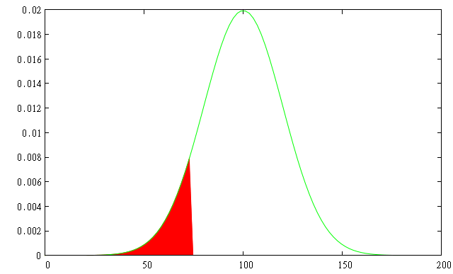
For listed products like stocks and bonds, we have enough historical data to evaluate the percentile based on that history. For more exotic products, like structure products, built on demand, prices are not available. In that case, prices are simulated and the same formula is then used like for historical values.
Monte-Carlo simulation
The method used is a computational algorithm based on random sampling. This technique is known as the Monte-Carlo method, by reference of the gambling games to the famous casinos in Monte-Carlo. To quickly describe how such method can lead to precise result with random values; let's see how to compute the number. Take a square with an edge length of 1.0 and a quarter of circle with radius length of 1.0 as in the schema thereafter. 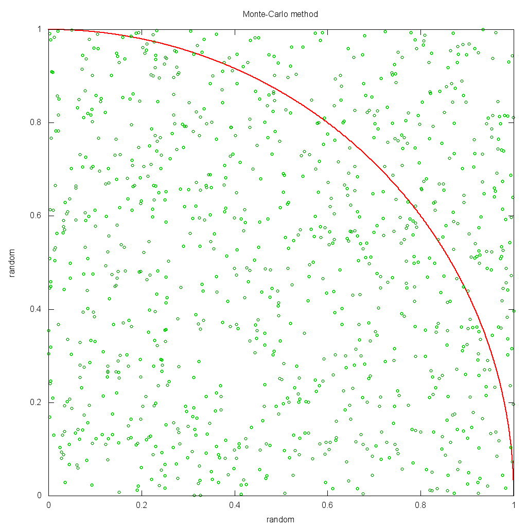
If you generate two independent random numbers x and y uniformly distributed between 0 and 1.0, it's like putting random dots on your square. With infinity of dots, the whole area is uniformly covered. The ratio between the number of dots in the circle () and the total number of dots equals the ratio between the areas of the quarter of the circle and the square. So }{1\times1}=\frac{\pi}{4}). The algorithm consists in generating random couples and counting the proportion of ranks in the circle. Multiplying it by 4 gives an approximation of the number.
For financial purpose, we will replace random dots by random simulations of market parameters (such as underlying price, interest rate) and the circle area by a predictable model allowing computing the portfolio value with these parameters.
A simple example: portfolio with one call
For the purpose of this article, I chose a very simple portfolio with only one product: a long position on a call (i.e. the owner has bought a call). A call is an option of buying, a financial contract giving the right but not the obligation to the buyer to buy a certain quantity of a financial instrument (the underlying) at a given date (the maturity date) at a given price (the strike). The seller sells this contract for a given fee (the premium).
We can then build a first model of the payoff of this call according to the price that the underlying will have at maturity date (lets say in a year). 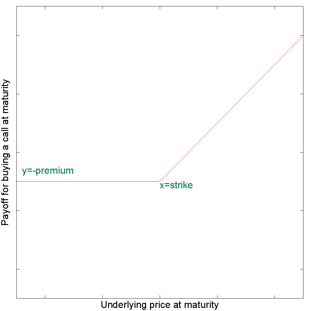
We now want to be able to build a model for the price of a call with a maturity in one year. But today we ignore the price of the underlying that might be in a year. I won't go deeper into details and will just say that a more complicated model exists. It is based on probability theory: the Black and Scholes model. It can determine the price of the call by knowing only:
- characteristics of the call : maturity date and strike price
- the price of the underlying as of today (and not anymore in the future)
- the risk free interest rate
- a parameter of the derivative market known as implied volatility.
The risk free interest rate can be estimated on Libor today's value (close to 5%). The underlying volatility can be deducted from listed options or from specific index like VIX and VAEX (see sample market values). In the example, we will take a value of 20. The Black and Scholes model for a single call can be expressed as a quite complex but closed formula (i.e. is predictable and can be easily computed). It is an arithmetic expression involving exp, sqrt and N(.) (cumulative distribution of normal distribution functions named NORMSDIST in Excel). See this Wikipedia article for more details and pay close attention to the available graphic which shows how the price of the option is modified when the price of the underlying is modified.
Estimation of the required computing power
By mixing these two methods, we can estimate the VAR for our sample portfolio. Required steps involved :
- Generating sample data for the three parameters that we have chosen: the underlying stock price, the interest rate and the underlying volatility. To keep it simple, we assume that these three parameters follow independent normal distributions.
- Calculating for each set of generated parameters, the corresponding option price according to the Black and Sholes expression
- Calculating the percentile at 1% for the distribution of option prices
Such individual computing is quite short but a large number of samples are required to get a correct precision of the end result. To give an order of magnitude, about 100,000 samples are required in our case. Using Excel 2007, on my laptop (a Dell Latitude with a core i7 with 2 multi-threaded cores and 4 GB RAM) 100,000 samples took approximately 2 s. for one option and one sample parameter simulated (underlying price). On the same laptop a mono-threaded Java program (using only one core) took about 160 ms. It seems to be quick but in real life, each exotic product in a portfolio is a combination of multiple options. A portfolio probably contains tens or hundreds of exotic products. Moreover, more complicated modeling is today used instead of Black and Scholes model requiring more complex calculation or more samples. So, the required computing power can easily get really huge.
The grid computing architecture

How to compute the VAR
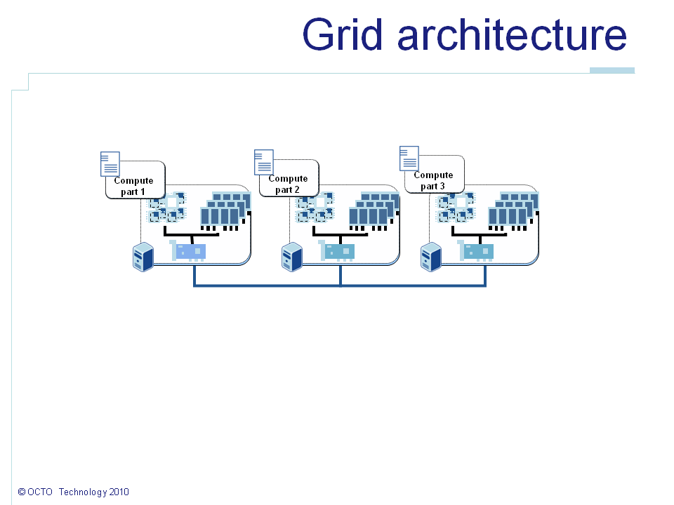
In order to be able to split, to distribute the VAR calculation, the algorithm should be adapted. The easiest way to get an approximation of the VAR of a portfolio could be by summing up the VAR of each product. The VAR of each product can be computed independently on each node. The algorithm can in that case remain unmodified. In the above schema, Compute part x corresponds to the calculation of an individual VAR. However, it will not allow speeding up the VAR calculation of our single call portfolio. And in a real life example, it would not allow us scaling up the number of samples so the precision.
Despite these flaws, lets see how we would implement it. We can use the map/reduce pattern. This pattern comes from functional programming where map m() list function applies the function m() to each element of the list, and reduce r() b list aggregates b parameter and all values of list into one single value. Lets take a practical example.
- The
map (\x -> 2*x) [1,2,3]returns[1*2,2*2,3*2]=[2,4,6]. - The
reduce (\x y -> x+y) 0 [2,4,6]returns0+2+4+6=12.
With such a pattern, the list can be split in N sub lists, sent to the N nodes of the grid. In that example, 1 is sent to the first node, 2 to the second, etc. The \x -> 2*x function code, sent with the values, is executed by each node: 2*1 by the first, 2*2 by the second, etc. You need to imagine that \x->2*x is replaced by a computer intensive function. Executing it in parallel will therefore divide the total required computing time. All results 2, 4, etc. are sent back to the sender node. The results are concatenated in the list [2,4,6] and the reduce (\x y -> x+y) is applied. The map function is split across nodes but not the reduce function which is executed by the sender node.
In our case, each sample generation will represent an element of the list. The map() function will, on each node, generate the sample data, compute the corresponding call price and return it. Then all call prices are sent to the reduce node. The reduce() function computes the percentile at 1% of the resulting data. Consequently it will give us the VAR at 99% of our portfolio. 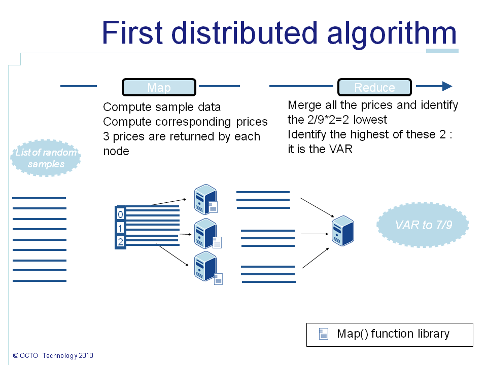
This first version works, but can still be a bit improved.
- First, the
reduce()function is not distributed, so it is better to minimize the amount of data it has to process. - Next, moving 100,000 prices over the network is resource consuming. In reality, network bandwidth is a scarce resource in a grid
Also we might notice that computing the percentile at 1% comes to sorting the data, and taking the highest value of the smallest 1% values. I presume that for the particular business case of this example the intermediate results can be discarded. In that case, this elimination algorithm can be distributed too. The idea is that the 10 smallest values of a set are included in the 10 smallest values of each of its subsets. Lets imagine that I'm looking up the 4 highest value cards of a poker deck. The deck has been split by suit into 4 sets. I can look in each set for the 4 highest cards. I will get an ace, a king, a queen and a jack for each suit. Then, I can merge these 4*4=16 cards and look again up the 4 highest ones. I will get the 4 aces. That can be generalized for any subsets.
So now, lets say we are computing 100,000 samples on two nodes. The percentile at 1% corresponds to the highest value of the 1,000 lowest values. On each node 50,000 values have been computed. On each node, we can take the 1,000 lowest values and send them as results instead of the 50,000. Then the reduce() function will only merge the two lists of the 1,000 lowest values, take the 1,000 lowest ones and identify the highest value. Indeed in the worst case where generated prices are totally sorted across nodes, the node with all the lowest values will give us the 1,000 lowest ones, guaranteeing that the percentile is still transmitted. Such optimization allows dividing by 50 the data that are transmitted thru the network. The benefit goes down when the number of nodes increases. In the worst case scenario, with 100 nodes there is no more benefit: each node has computed 1% of the data. But in practice, distributing small list of samples is counter-productive as distribution overhead is higher than the parallel computing gain. As you can see, these kind of business specific optimization ca really help minimizing the required resources.
The final algorithm is summarized in the following schema: 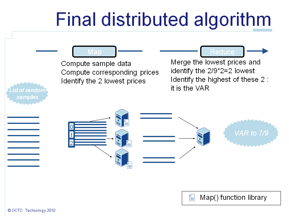
Conclusion
From a business point of view, risk estimation is becoming more and more important for financial institutions to prevent financial losses on fluctuant markets. Moreover, new regulation rules such as Basel III and Solvency II take into account the VAR in their requirements. Computing efficiently such figures is a key requirement for Information System of financial institutions. Through a very simple example, this article has shown that such calculation consists in generating sample data, doing some mathematical processing to compute a value for the portfolio for each sample data. The amount of sample data and sometimes the complexity of the processing require specific architectures to finish such calculations in a reasonable time. Grid computing is the most up-to-date architecture to solve these problems. Using map reduce pattern is one of the easiest way to write an algorithm that benefitiates of grid computing parallel capabilities. Also, business requirements understanding is a key point in optimizing the code. In this example, dropping the intermediate results allows to speed up the calculation. In another article, I will describe an implementation of that example using a grid computing middleware and will give some performance figures.