D3.js certainly is the most versatile JavaScript data rendering library available: turning data into mind blowing visualizations is only limited by your imagination. A key component to turn static pages into animated ones are the powerful selection transitions. However, too many simultaneous transitions on a web page will soon bring you CPU on its knees. Hence this blog post.

We faced this problem when displaying swiss transport real time data on a map, within an SVG layout: rendering was lagging, event sourced data were not consumed consistently and laptop batteries were drowning at a dramatic speed. A video from a first attempt can be seen, and compared to a newer implementation with the technique presented in this article. Another surprise came from rendering a simple clock, burning 20% of CPU with a single transition.

If d3.js has no serious concurrents for many rendering problems, we decided to give try to a JavaScript library used for building games and leveraging the strengths of HTML5 and GPU: pixi.js.

At first, we will propose in this post a comparison between the two libraries in terms of rendering performance. For the sake of completeness, we will also discuss native CSS transitions. We will then dive into a couple of tricks to enhance dynamic visualizations with each of the two libraries and will even combine them to get the best of both worlds.

The project source code with benchmark data are hosted on github and a demo is available on github.io.

Experimental Setup

To simulate a simple system with many transitions, we built a model with three parameters. n particles are randomly scattered in  a 2D box. Every dt milliseconds, a new random relative position is attributed for each particle. Particles cannot exit the box and the average leap length for the next move is the third model parameter.

The transition type we will focus in this experiment are linear ones, but the same phenomenon can be observe with others (rotations, opacity, scaling etc.)

The project source code makes a vanilla use of  Angular 2 and ngrx/store to implement a flux pattern. A store handles the particles state at each dt interval and the rendering components subscribe to an observable to react upon changes. The transitions themselves are managed by the rendering components.

Measures are mainly done on Chrome v55, running on a Macbook pro (2015, 2.5Ghz i7, 16G RAM). Several metrics were captured:

• CPU: via task manager, allowing tab centric monitoring;
• GPU: via task manager “GPU process”;
• number of frames per second (FPS): via the developer console rendering tab;
• cycle time: if new particle positions are set by the store every 1000 milliseconds, we also want to measure the time between two actual rendering iterations. In a perfect world, it should be 1000ms + epsilon, epsilon being the time for computing those new positions and setting up the transition mechanism. This measure is captured via console log, where the current time minus the one at the previous iteration is displayed.

Transition implementations

As most of the implementation is a straightforward Angular 2 + ngrx/store use, we will  focus only on the transition part.

D3.js [code] [simulation]

D3.js core strength is to tie a data structure to DOM elements and opens the doors for rich visualization. In our case, an array of particles are associated with circles within an SVG element. The association between the x and y particle properties and the cx and cy circle attributes is achieved via an update pattern:

self.svg.selectAll('circle')      .attr('cx', function (b) {        return self.width * b.x;      })      .attr('cy', function (b) {        return self.height * b.y;      });

One of the great “magic” of d3.js is the ability not only to modify a DOM element attribute at once, but to make it transition from its current value to the new one via  continuous transitions. This mechanism is set in the following example by three calls:

self.svg.selectAll('circle')      .transition()      .duration(1000)      .ease(d3.easeLinear)      .attr('cx', function (b) {        return self.width * b.x;      })      .attr('cy', function (b) {        return self.height * b.y;      });

Et voilà!

Pixi.js [code] [simulation]

Pixi.js is a library to render 2D animation. It benefits from HTML5 features and leverages the power of the WebGL rendering engine. The library success comes from the proposed abstraction above the classic low level implementation details. Even though its “market share” is more turned toward online games, we will demonstrate here how it can also play a role in data visualization.

Pixi.js documentation is rather comprehensive, so we will not cover here the full implementation story. Each particle is tied to a Graphics circle object. The original and target positions are stored and the actual coordinates are updated via a requestAnimationFrame call.

const tFrom = new Date().getTime();    const animate = function () {      const tRatio = (new Date().getTime() - tFrom) / 1000;      if(tRatio>1){        return;      }      for (let i = 0; i < n; i++) {        let g = self.graphics[i];        g.x = g.xFrom + tRatio * (g.xTo - g.xFrom);        g.y = g.yFrom + tRatio * (g.yTo - g.yFrom);      }      self.renderer.render(self.stage);      requestAnimationFrame(animate);    };    animate();

Results

Benchmark data was collected as described in the experimental setup section and processed with R. The analysis notebook code (knitr) is available [here].

CPU and GPU

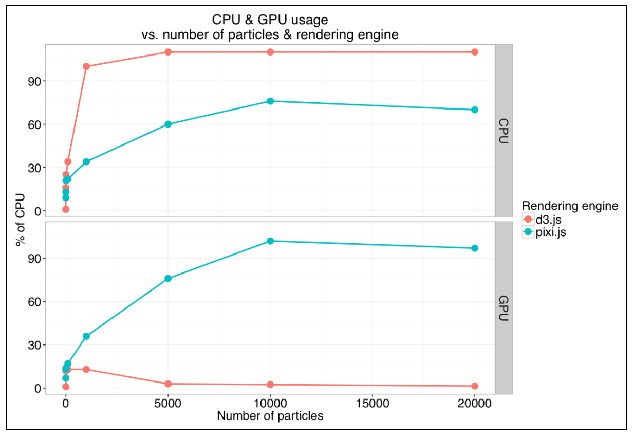
Figure 1: CPU & GPU measured usage are displayed versus the number of particles in the box. Both rendering engines are compared.

Figure 1 shows CPU & GPU consumptions, depending on the number of particles moving across the screen. Those numbers confirm the intuition based on CPU monitoring (or simply feeling the laptop fan striving): as soon a a few hundred particles are transitioned simultaneously, CPU peak is reached. Moreover, we can confirm that D3 transitions do not use any GPU power to slim the process. On the contrary, Pixi, using HTML5, hits the CPU much lighter and leverages GPU to gain efficiency. With this later approach, up to 10’000 particles can be moved comfortably. It can also be noted that even a single particle being transitioned already consume 16% of CPU! Of course, CPU is flat when no particles are displayed).

Frame per seconds & cycle time

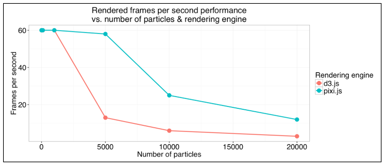
Figure 2: the number of frames rendered per seconds, as indicated by the Chrome developer console. If 60 is the peak value, lagging is perceived with rates below 20 FPS.

Another intuition is confirmed: when more are present, the particle movements starts to be jerky. The number of frames rendered per second diminishes much sooner with d3.js than with Pixi. Even with more than 10’000 particles, Pixi sustains a rate greater than 20 frames per second, hence a comfortable experience for visualization.

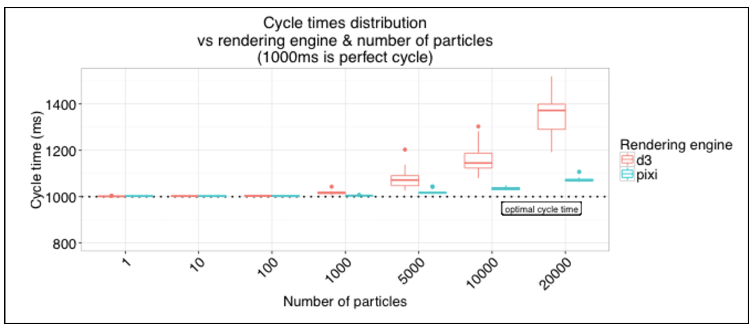
Figure 3: the effective time between two loop is displayed as a box plot, as several measures were collected for each situations. A “costless” situation prduces cycle times at 1000 ms. We can see the measures diverging as soon as the number of particle reaches 1000, with a clear disavantage to D3.

Finally, looking at the cycle time nails the point, as shown in figure 3. As the CPU is harassed by transitions, it cannot be used as efficiently to address the other tasks, such as computing the next particle positions (or in real life, all the other tasks to be taken care of). This induces lags between each simulation steps and therefore less smooth animations. This phenomenon is of course less intrusive with Pixi.

Enlarging the scope

Other measures are not presented here. We made simulations to see if semi transparent objects would impact performances, but the alpha factor proved to have no effect. Looking at other transition types (e.g. rotations, scaling) did not raise contradictory effects neither.

For the sake of the exploration, we also considered using Pixi without enabling the WEBGL, and falling on a canvas renderer. Results are not displayed here (thus they are available on github), but this third option falls as an intermediary between the two solutions proposed in this post.

To broaden the browser range, an attempt to benchmark Firefox (v49) was done, but the lack of comfortable tooling did prevent us to pursue this goal. However, approximative measures gave the same kind of outcome as with Chrome.

Wait! Why didn’t you use native CSS transitions? [code] [simulation]

Among the first comments to this post was the question: “d3.js does not use native CSS transitions. Wouldn’t they be more appropriate for your problem?”

CSS indeed proposes native transitions, that can, in some conditions leverage the GPU.

We use d3 to set the CSS transitions, as shown in the code below . A check has be done with only setting the translation with CSS + D3, without transition effect: CPU levels is neglectable, proving the lack of an eventual overhead by D3.

self.svg.selectAll('circle')      .data(self.particleSet.particles, function (b) {        return b.id;      })      .enter()      .append('circle')      .attr('r', 2)      .attr('cx', 0)      .attr('cy', 0)      .style('transition-timing-function','linear')      .style('transition-duration', '1000ms')

self.svg.selectAll('circle')      .style('transform', function(b){        return 'translate('                +(self.width * b.x) + 'px, '                +(self.height * b.y) + 'px)';      })

Unfortunately, if transitions can be described in CSS for SVG, figure 4 shows that performance are even poorer than those with D3.

But what about the claim of CSS transitions using the GPU? We made another experiment, with particles displayed as <div> moving on the screen [code] [simulation]. In this situation, GPU is effectively triggered, with better performance although lower than Pixi’s. However, the alternative of stepping out from the SVG container lays outside of the original problem at hand.

Figure 4: a duplicate from figure 1, with native SVG CSS transitions. They show to be slightly worse than D3 selection transitions.

More & better rendering

Limiting d3.js transitions [code] [simulation]

We have seen how with D3, the CPU is loaded by selection transitions. In practical situations such as simulating public transport vehicles, some moves may be shorter than others. If the leap is below 2 pixels of distance per time increment, a continuous transition is not necessary and may be replaced by an atomic jump without too much visual impediment.

From the implementation point of view, it is a matter of filtering particles with jumps smaller or larger than 2 pixels and applying either an instantaneous modification or calling for a transition.

//add a delta property as the leap distance      self.svg.selectAll('circle')      .each(function (b) {        b.delta = Math.max(Math.abs(b.xFrom - b.x) * self.width,                           Math.abs(b.yFrom - b.y) * self.height);        });

//a direct jump is applied if the distance is lower than 2      self.svg.selectAll('circle')        .filter(function (b) {          return b.delta <= 2;        })        .attr('cx', function (b) {          return self.width * b.x;        }); //and so with 'cy'

  // a linear transition is triggered in other situations

self.svg.selectAll('circle')        .filter(function (b) {          return b.delta > 2;        })        .transition()        .duration(1000)        .ease(d3.easeLinear)        .attr('cx', function (b) {          return self.width * b.x;        }); //and so with 'cy'

The impact on CPU is directly linked to the number of objects filtered out from the transition loop.

Adding tail effect with Pixi.js [code] [simulation]

Pixi let us step into the gaming world, where transitions effect can be enhanced. A classic way to do so is to add a fading out tail to each particle. Pixi allows to render a scene to the window, but also to a background texture. One trick is to render the latest stage to the screen, then add  the full stage to a buffered texture by adding a light opacity effect.

self.stage.addChild(self.outputSprite); //and within the animation loop      const temp = self.renderTexture;      self.renderTexture = self.renderTexture2;      self.renderTexture2 = temp;      self.outputSprite.texture = self.renderTexture;

self.renderer.render(self.stage);      self.stage.alpha=0.8;      self.renderer.render(self.stage, self.renderTexture2); //turn the stage opacity back to 100%      self.stage.alpha=1;

Such a texture superposition has been measured to have little overall performance impact.

Combining Pixi & D3: the best of both worlds [code] [simulation]

For massive transitions, Pixi has clearly proven its value. But it can hardly replace the power and versatility of D3 for other types of complex visualizations. For the sake of the example, we proposed to add a circle below the Pixi scene. The center shows the average particle positions while the radius shows the standard deviation of the distance to this center. Therefore, the circle attributes are also to be recomputed at every time increment.

The method proposed in the previous section ensures the stage background to be transparent (to the contrary of other Pixi tailing effect methods proposed on the web).

We simply used two <div> elements  to superimpose a D3 and a Pixi layers.

But everything is not only about speed

Even though we have focused on performance issues, we shall not close this discussion without mentioning a few points worth remembering when comparing the two libraries:

• d3.js extends far beyond moving a few circles across an SVG box. Its real power comes with the possibility to interact with any element, CSS and the vast toolbox made available.
• Pixi.js offers other abstractions to manipulate a lot of similar objects (SpriteBatch et ParticleContainer). These tools are particularly well suited to render a large fixed number of images.
• Another advantage of Pixi is to asynchronously add or remove elements to the stage. Although it is not demonstrated in the current example, we can use this pattern to tie objects to a data stream (think of Server Side Events).
• No easy solution seems to exists to throttle d3 transitions (even though mist.io proposed an alternative) . It is however rather straightforward to implement such a throttle in a Pixi animation loop.
• The focus on massive transitions in this post shall not make us that there are more than one way to do animation. Head for Bourbon.io and snap.svg to rock!

Conclusions

No doubt Pixi is more efficient to render a lot of transitions! As soon as the number of objects reaches a few hundreds, aiming to such a technology should seriously be considered. Even though the Pixi coding part is not as straightforward as D3, it leverages the power of the GPU cards, available on any modern computers. But the versatility of D3 to render the vast majority of other graph types makes it hard to forget (think of drawing maps with topojson or any plot indicators).

The good news therefore comes by the easiness to combine both approaches. D3 scales can even be used from inside Pixi code to benefit from a coherent domain to screen coordinates system.

Coming soon...