The basics of face recognition

Face Recognition is definitely one of the most popular computer vision problems. Thanks to its popularity it has been well studied over the last 50 years. The first intents to explore face recognition were made in the 60's however it was until the 90's when Turk and Pentland implemented the "Eigenfaces" algorithm, that this field showed some really exciting and useful results.

Bright future

Face recognition is recently getting more and more attention and we can anticipate bright future of this field.

Security was historically and will stay in the future the main application of face recognition in practice. Here face recognition can help with both: identification and authentication. Good example is the Frankfurt airport security system which uses face recognition to automatize passenger control. Another application can be the security analysis of videos purchased by external city cameras systems. Potential suspects can get identified before committing crime. Take a look at the integration of face recognition to London Borough of Newham, already in 1998.

Face recognition can be also used to speedup the identification of persons. We can image a systems which would recognize the client as soon as he walks into branch store (bank, assurance), and the front-office worker can than welcome the client by has name and prepare his folder before he actually gets to the counter.

Advertising companies are working on ad-boards which would adapt their content to the persons passing by. After analyzing the persons face, commercials would adapt to the gender, age, or even personal style. This usage however, might not conform to privacy laws. Private companies do not have rights to film persons in public places (of course, depending on the country.

Not to forgot, that Google and Facebook had both implemented algorithms to identify users in the huge database of photos which they maintain as part of their social network services. Third party services, such as Face.com offer Image base searching, which allow you search for example for picture which contain together your best friends.

One of the latest usages is coming also from Google and it is the Face Unlock feature, which will as the name says, enable you to unlock your phone after your face has been successfully recognized.

Latest news come to face recognition thanks to new hardware equipment, specially 3D cameras. 3D cameras obtain much better results, thanks to their ability to obtain three dimensional image of your face and solve problems which are the main issues in 2D face recognition (illumination, background detection). See the example of Microsoft Kinect , which can recognize you as soon as you walk in front of the camera.

We should keep in mind, that face recognition will be used more and more in the future. This applies not only to face recognition, but to the whole field of machine learning. The amount of data generated every second forces us to find ways to analyze the data. Machine learning will help us to find a way to get meaningful information from the data. Face recognition is just one concrete method from this big area.

How to get started?

Several methods and algorithms were developed since than, which makes the orientation in the field quite difficult for the developers or computer scientists coming to face recognition for the first time.

I would like this article to be a nice starter to the subject which will give you three pieces of information:

• What are the algorithms and methods used to perform face recognition.
• Fully describe the "Eigenfaces" algorithm.
• Show a fully functional example of face recognition using EmguCV library and Silverlight Web Camera features. Go directly to the second part of this article, describing the implementation.

Face recognition process

The process of recognizing a face in an image has two phases:

• Face detection - detecting the pixels in the image which represent the face. There are several algorithms for performing this task, one of these "Haar Cascade face detection" will be used later in the example, however not explained in the article.
• Face recognition - the actual task of recognizing the face by analyzing the part of the imaged identified during the face detection phase.

Face recognition brings in several problems which are completely unique to this domain and which make it one of the most challenging in the group of machine learning problems.

• Illumination problem - due to the reflexivity of human skin, even a slight change in the illumination of the image can widely affect the results.
• Pose changes - any rotation of the had of a person will affect the performance.
• Time delay – of course that due to the aging of the human individuals, the database have to be regulary updated.

Methods and algorithms

• Apearance based statistical methods are methods which use statistics do define different ways how to measure the distance between two images. In other words they try to find a way to say how similar two faces are to each other. There are several methods which fall into this group. The most significant are:

  • Principal Component Analysis (PCA) - described in this article.
  • Linear Discriminant Analysis (more information)
  • Independent Component Analysis (more information)

  PCA is described in this article, others are not. For comparison of these methods refer to this paper

• Gabor Filters – filters commonly used in image processing, that have a capability to capture important visual features. These filters are able to locate the important features in the image such eyes, nose or mouth. This method can be combined with the previously mentioned analytical methods to obtain better results.

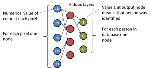
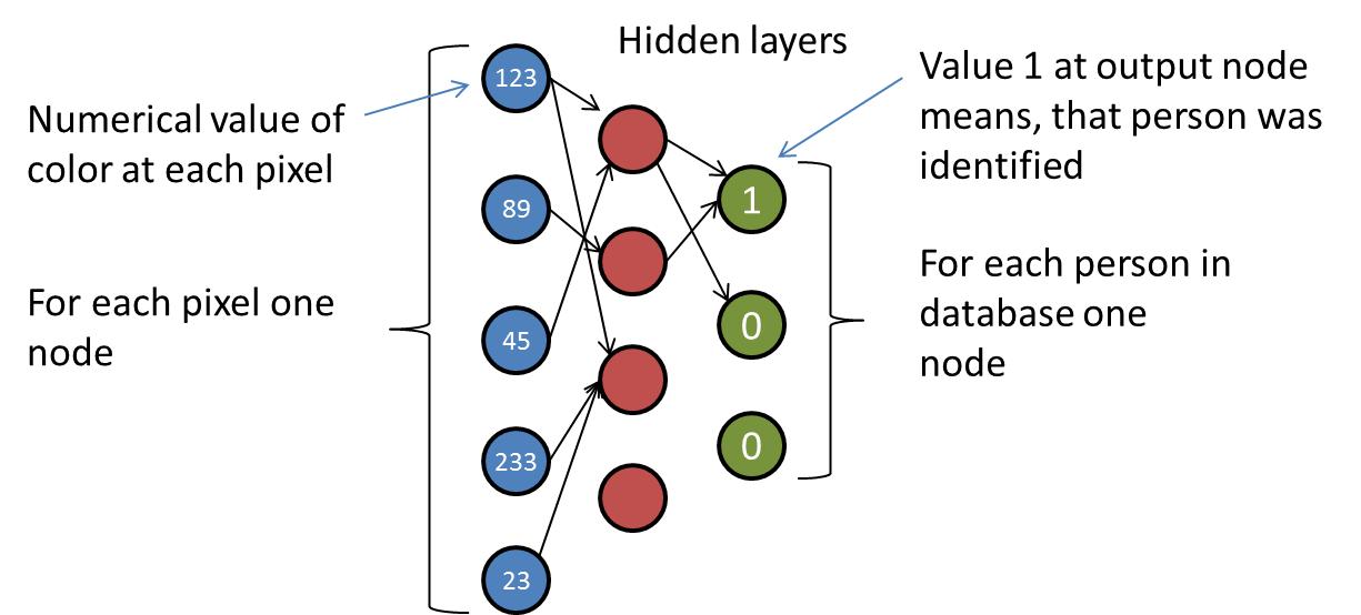
• Neural Networks are simulating the behavior of human brain to perform machine learning tasks such as classification or prediction. In our case we need the classification of an image. The explication of Neural Networks would take at least one entire article (if not more). Basically Neural Network is a set of interconnected nodes. The edges which are between the nodes are weighted so the information which travels between two nodes is amplified. The information travels from set of input nodes, across a set of hidden nodes to a set of output nodes. The developer has to invent a way to encode the input (in this case an image) to a set of input nodes and decode the output (in this case a label identifying the person) from the set of output points. Commonly used method is to take one node for each pixel in the image on the input side of the network and one node for each person in the database on the output side as ilustrated on the following image: For more information about face recognition using Neural Networks visit this link

Eigenfaces algorithm and PCA

The eigenfaces algorithm follows the pattern which is followed by other statistical methods as well (LDA, ICA):

1. Compute the distance between the captured image and each of the images in the database.
2. Select the example from the database, which is closest to the processed image (the one with the smallest distance to captured image).
3. If the distance is not too big – label the image as concrete person.

What is the distance between two images?

The crucial question is: How to express the distance between two images? One possibility would be to compare the images pixel by pixel. But we can immediately feel, that this would not work. Each picture would contribute the same to the comparison, but not each pixel holds valuable information. For example background and hair pixels would arbitrary make the distance larger or smaller. Also for direct comparison we would need the faces to be perfectly aligned in all pictures and we would hope that the rotation of the head was always the same.

To overcome this issue the PCA algorithm creates a set of principal components, which are called eigenfaces. Eigenfaces are images, that represent the main differences between all the images in the database. The recognizer first finds an average face by computing the average for each pixel in the image. Each eigenface represents the differecens from the avarage face. First eigenface will represent the most significant differences between all images and the average image and the last one the least significant differences.

Here is the average image created by analyzing the faces of 10 consultants working at OCTO Technology, having 5 image of each consultant.

And here are the first 5 Eigenfaces:

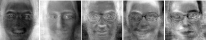
Note that the consultants at OCTO are generally handsome guys and this ghost-look is characteristic to the eigenfaces of any group of persons. You can also notice that there is one face which is dominant. That is due to the fact that I had just limited number of pictures of my colleges and I could take a lot of myself using web cam. This way my face become a little dominant over others.

Now when we have the average image and the eigenfaces, each image in the database can be represented as composition of these. Let’s say:

Image1 = Avarage Image + 10% Eigenface 1 + 4% Eigenface 2 + … + 1% Eigenface 5

This basically means that we are able to express each image as a vector of percentages. The previous image becomes to our recognizer just a vector [0.10, 0.4, … , 0.1]. The previous equation is a slight simplification of the subject. You might be asking yourself how are the coefficients of each eigenface computed. If we would enter into the details,

Now when we have expressed the image as a simple vector, we are able to say what is the distance between two images. Getting the distance of two vectors is not complicated and most of us remember it from school.

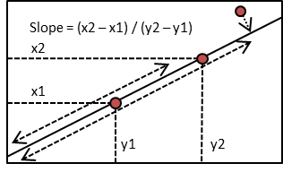
If in 2D space we have the vectors [x1,y1] and [x2,y2] we now that the distance between these two can be visualized and computed as shown in the following picture:

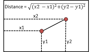
Now we can perform similar calculation for the vectors which represent our images.

Behind the scenes

This part will give you some more insights into how exactly are the eigenfaces computed and what is going on behind the scenes. Feel free to skip it if you do not want to enter more into the details.

The key point in the PCA is the reduction of dimensional space. The question we could pose us is, how would we compare the images without eigenfaces. We would simply have to compare each pixel. Having and image with resolution 50 x 50 pixels, that would give us 2500 pixels, in other words we would have space of 2500 dimensions. When comparing using the eigenvalues we arrived to reduce the dimensional space – the number of eigenfaces is the number of dimensions in our new space.

Remember the equation of the distance of two points – now in this equation each pixel would contribute to the distance between images. But not each pixel holds some meaningful information. The background behind the face, the cheeks, the forehead, hairs – these are the pixels which do not give meaningful information about the face. Instead the eyes, nose, ears are important. In the terms of Image processing lot of pixels just bring noise to the computation of the distance. One of the main ideas of PCA is the reduction of the noise by reducing the number of the dimensions.

Reducing the number of dimensions

You may be asking yourself, how exactly can we reduce the number of dimensions? It is not easy to imagine the transition from a space where each pixel is one dimension to a space where each eigenface is one dimension. To understand this transition, take a look at this example:

In two-dimensional space, each point is defined by its two coordinates. However if we know, that several points lay on the same line, we could identify the position of each point only by knowing it's position along the line. To obtain the x and y coordinate of the point we would need to know the slope of the line and the position of the point on the line. We have reduced the dimension by one. In this example the slope of the line becomes the principal component, the same way our eigenfaces are principal components during the face recognition algorithm. Note that we can even estimate the position for the points which are not on the line, by using the projection of the point on the line (the case of the last point).

From mathematical point of view eigenfaces are graphical representation of eigenvectors (sometimes called characteristic vectors) of co-variance matrix representing all the images. That it how they got their name. For more details on Principal Component Analysis and computation of eigenvectors and eigenfaces visit the following links: PCA and Eigenvectors

Isn't there an easy way?

You might be thinking, that this is too complex as introduction to the subject and you might be asking yourself whether there is an easy way to start with face recognition?

Well yes and no. Eigenfaces algorithm is the base of the research done in face recognition. Other analytic methods such as Linear Component Analysis and Independent Component Analysis build on the foundations defined by the eigenfaces algorithm. Gabor filters are used to identify the important features in the face and later eigenfaces algorithm can be used to compare these features. Neural Networks are complex subject, but it has been shown that rarely they have better performance then eigenfaces algorithm. Sometimes the image is first defined as linear combination of eigenfaces and than it's describing vector is passed to the Neural Network. In other words eigenfaces algorithm builds really the base of face recognition. There are several open-source libraries which have implemented one or more of these methods, however as a developers we will not be able to use them without understanding how these algorithms work.

Enough of theory now! Visit the second part of the article to see how to include face recognition into your web application.